Training Compute-Optimal Large Language Models

We investigate the optimal model size and number of tokens for training a transformer language model under a given compute budget. We find that current large language models are significantly undertrained, a consequence of the recent focus on scaling language models whilst keeping the amount of training data constant. By training over 400 language models ranging from 70 million to over 16 billion parameters on 5 to 500 billion tokens, we find that for compute-optimal training, the model size and the number of training tokens should be scaled equally: for every doubling of model size the number of training tokens should also be doubled. We test this hypothesis by training a predicted compute-optimal model, Chinchilla, that uses the same compute budget as Gopher but with 70B parameters and 4\times more more data. Chinchilla uniformly and significantly outperforms Gopher (280B), GPT-3 (175B), Jurassic-1 (178B), and Megatron-Turing NLG (530B) on a large range of downstream evaluation tasks. This also means that Chinchilla uses substantially less compute for fine-tuning and inference, greatly facilitating downstream usage. As a highlight, Chinchilla reaches a state-of-the-art average accuracy of 67.5% on the MMLU benchmark, greater than a 7% improvement over Gopher.

Five Important Things

1. Optimal Parameter/Training Tokens Allocation

Suppose one day your boss comes up to you and says “management has allocated you \(C\) compute units to train a large language model, godspeed” and now you need to figure out what Transformer model parameters to use and how big your dataset should be to get the best possible perplexity.

This paper (also known as the Chinchilla paper) builds up on the work from Kaplan et al. 2020, noting that the scaling laws do hold but obtaining different constants.

They performed several experiments to understand the scaling laws, the subject of the next few sections.

2. Approach 1: Fix Model Sizes and Vary the Number of Training Tokens

The authors used a range of model sizes from 70M to 10B, and plotted the loss achieved against training tokens used (leftmost plot below):

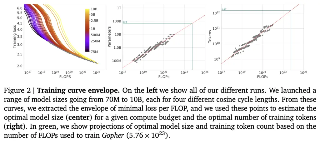
For each level of loss, they then took the parameter count and token count of the model that required the least number of FLOPs, giving rise to the middle and right plots above.

This allowed them to verify the power law for numbers of parameters against compute \(N_{\mathrm{opt}} \propto C^a\), and the size of the dataset against compute \(D_{\mathrm{opt}} \propto C^b\).

3. Approach 2: IsoFLOP Profiles

In this approach, they fixed the total compute budget available at 9 different levels, and experimented with the final loss achieved by varying model sizes at each level.

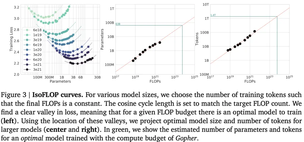
With reference to the left diagram above, each curve represents model sizes along the same compute budget. The curves are U-shaped, and the model run on the lowest point for each of the “valleys” is taken and used to produce the middle and right plots.

These curves allowed them to fit \(N_{\mathrm{opt}} \propto C^a\) and \(D_{\mathrm{opt}} \propto C^b\) with roughly the same constants as Approach 1.

4. Approach 3: Parametric Fitting of the Loss

The authors propose the following functional form for the loss:

\[\hat{L}(N, D) \triangleq E+\frac{A}{N^\alpha}+\frac{B}{D^\beta}\]

The first term \(E\) is the entropy of the text, which is the minimum loss achievable. The other two terms model the power law relationship with \(N\) and \(D\).

The way that they derived this functional form is by the standard empirical risk decomposition.

The Bayes classifier \(f^\star\) achieves the best possible cross-entropy loss, given by \(L(f) \triangleq \mathbb{E}\left[\log f(x)_y\right]\). This is the same as \(E\) from above.

In our setup, we restrict ourselves to the hypothesis class of Transformers of size \(N\) denoted by \(\mathcal{H}_N\). Then the best possible model is \(f_N \triangleq \underset{f \in \mathcal{H}_N}{\operatorname{argmin}} L(f).\)

However, when training our Transformer, we do not have access to the data distribution but only the empirical distribution (i.e training data), and hence we can only compute the surrogate objective of the empirical loss \(\hat{L}_D(f) \triangleq \hat{\mathbb{E}}_D\left[\log f(x)_y\right]\). Then the theoretically optimal Transformer that we can get is \(\hat{f}_{N, D} \triangleq \underset{f \in \mathcal{H}_N}{\operatorname{argmin}} \hat{L}_D(f)\).

But even this is too strong - in practice, we don’t train to convergence or know that we have achieved the lowest possible loss, and hence we denote the actual single-epoch empirical-risk minimizer trained by stochastic gradient descent by \(\overline{f}_{N,D}\).

Then now we can write

\[\begin{align*} L(N, D) & \triangleq L\left(\bar{f}_{N, D}\right) \\ & = L\left(f^{\star}\right)+\left(L\left(f_N\right)-L\left(f^{\star}\right)\right)+\left(L\left(\bar{f}_{N, D}\right)-L\left(f_N\right)\right). \\ & \text{(adding terms that cancel each other, and rearranging)} \end{align*}\]

The first time corresponds to \(E\)
The second term models the excess risk due to restrictions on the function class and corresponds to \(\frac{A}{N^{\alpha}}\), where we see that as \(N\) increases, it becomes more expressive and hence the excess risk decreases
The last term models the excess risk due to optimizing over the empirical distribution instead of the data distribution, which corresponds to the term \(\frac{B}{D^\beta}\). Again, we see that as we increase \(D\), this excess risk decreases since it converges to the data distribution.

By fitting the data to the functional, the authors recovered the coefficients

\[L(N, D)=E+\frac{A}{N^{0.34}}+\frac{B}{D^{0.28}}.\]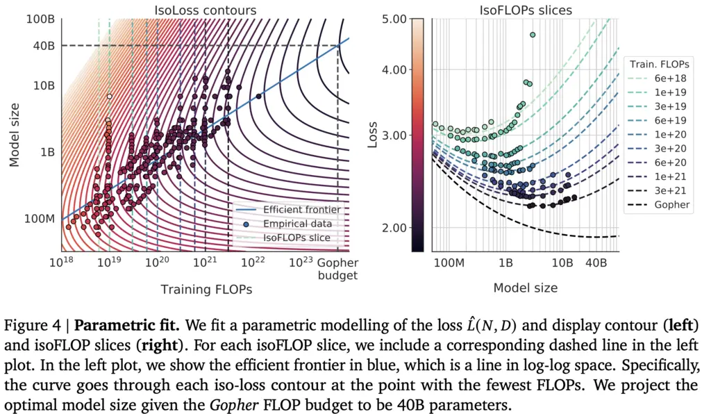

With reference to the left plot above, each of the dotted vertical lines represents each of 9 FLOPS levels, plotted against model size. Each of the curves in the graph represents contour lines of the same level of loss, from higher loss in the lighter regions near the bottom left (corresponding to smaller models and fewer FLOPs), to lower loss in the darker regions on the top right (corresponding to larger models and higher FLOPs).

The blue line of the efficient frontier then denotes the turning points for each of these curves, denoting the minimum model size and FLOPs required at each loss level.

The right graph shows the same data in another way, by showing for each compute budget, the loss that can be achieved with different model sizes.

5. Chinchilla

To put their findings to the test, the authors trained a LLM with the same compute budget as Gopher (280B), but using the optimal model size (70B) and amount of data (4x more).

They found that the compute-optimal Chinchilla outperformed Gopher substantially over most downstream evaluation tasks.

Most Glaring Deficiency

It would have been good if the authors also replicated and investigated the invariance of the scaling laws across different model parameters (number of attention heads, number of Transformer blocks, etc).

Conclusions for Future Work

The paper was well-motivated and easy to read, and provides further empirical evidence for neural scaling laws. It gives researchers another set of guidelines on how model parameters should be selected.