Scaling Laws for Neural Language Models

We study empirical scaling laws for language model performance on the cross-entropy loss. The loss scales as a power-law with model size, dataset size, and the amount of compute used for training, with some trends spanning more than seven orders of magnitude. Other architectural details such as network width or depth have minimal effects within a wide range. Simple equations govern the dependence of overfitting on model/dataset size and the dependence of training speed on model size. These relationships allow us to determine the optimal allocation of a fixed compute budget. Larger models are significantly more sample-efficient, such that optimally compute-efficient training involves training very large models on a relatively modest amount of data and stopping significantly before convergence.

Four Important Things

1. Power Law Relationship of \(L\) With Respect To \(N, C, D\)

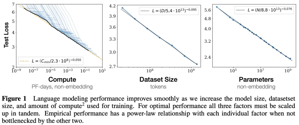
The paper shows empirically that language modeling loss \(L\) is a predictable function of:

\(N\), the number of model parameters (excluding embeddings).
\(D\), the size of the dataset,
\(C\), the amount of compute used for training,

when they are not bottlenecked by any of the other two parameters.

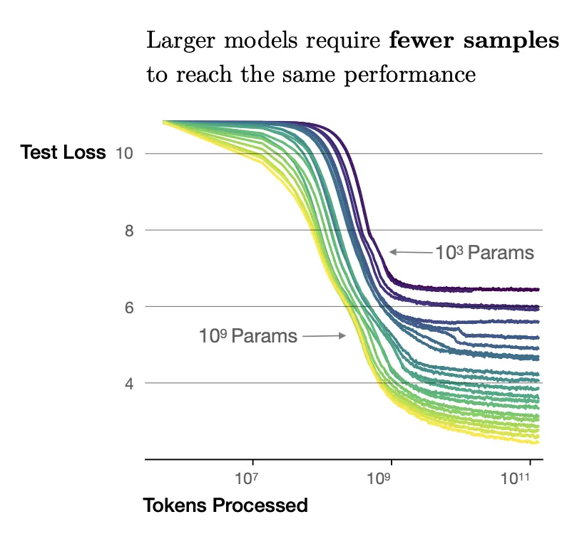
The paper also observed that larger models are more sample-efficient than smaller models, being able to reach the same loss with fewer samples.

In the graph below, we see that the curves corresponding to the \(10^9\) parameter model achieves a much smaller test loss compared to the \(10^3\) parameter model at all regimes:

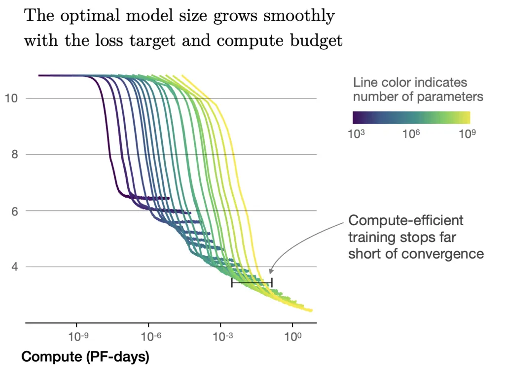
In addition, they surprisingly found that for a fixed compute budget and no restrictions on model size or available data, the optimal loss that can be achieved is not by training a model to convergence, but rather training a very large model that significantly stops short of convergence. One’s intuition for smaller models would be that models should be trained to convergence, and this often happens in practice due to hardware constraints.

In the graph below, we see that the curves flatten out towards the end with increasing compute, which provides intuition on why it is preferable to over-parameterize the model further in order to stay within the non-flattening regime of decaying test loss:

2. Transformer Performance Depends Weakly on Shape Parameters

We parameterize the Transformer architecture by the following hyperparameters:

\(n_{\textrm{layer}}\), the number of Transformer block layers
\(d_{\textrm{model}}\), the dimension of the residual stream (i.e the dimensions output by the residual connection and layer normalization components, which is the dimension preserved between each Transformer block)
\(d_{\textrm{ff}}\), the dimension of the feed-forward layer
\(d_{\textrm{attn}}\), the dimension of the attention output
\(n_{\textrm{heads}}\), the number of attention heads per layer

To jolt your memory of how these different components come together again, here’s the original Transformer architecture from Vaswani et. al:

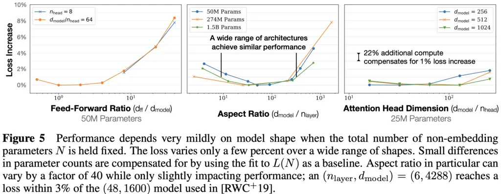
The authors showed that the performance of Transformers only depends weakly on \(n_{\textrm{layer}}\), \(n_{\textrm{heads}}\), and \(d_{\textrm{ff}}\) when the total number of parameters is held fixed. It was not elaborated what “weakly” means precisely, but I understood it to mean that the relationship is something that would be swallowed in the context of big-O analysis.

To study the relationships of performance on these hyperparameters, they always scaled \(d_{\mathrm{model}}\) accordingly to keep \(N \approx 12 n_{\mathrm{layer}} d_{\mathrm{model}}^2\) fixed. \(d\_{\mathrm{model}}\) controls the width of the Transformer, and makes sense to be the one modified since it can allow the most significant parameter. changes without changing its own value too significantly.

(Right plot) For \(n_{\mathrm{heads}}\), we see that loss increases as \(n_{\mathrm{heads}}\) decreases, but this can be offset by increasing \(d_{\mathrm{model}}\), which leads to their remark in the plot.
(Middle plot) For \(n_{\mathrm{layer}}\), as the number of layer decreases and \(d_{\mathrm{model}}\) increases, the loss increase goes down and then goes up again across a range of architectures with different \(N\). This means there is a sweet spot for trading off between the two parameters.
(Left plot) For \(d_{\mathrm{ff}}\), as \(d_{\mathrm{ff}}\) increases and \(d_{\mathrm{model}}\) decreases, the increase in loss goes down slightly, before growing a lot more. This also hints at a sweet spot between the two parameters.

The fact that the loss only weakly depends on model shape is desirable since it makes the analysis of scaling laws more robust (minor changes in architecture should not result in major changes in the results, much like how minor tweaks to the Turing machine architecture should not change asymptotic analysis significantly).

3. Comparisons with LSTMs

It would be interesting to understand how the scaling laws of Transformers compare to the classical LSTM.

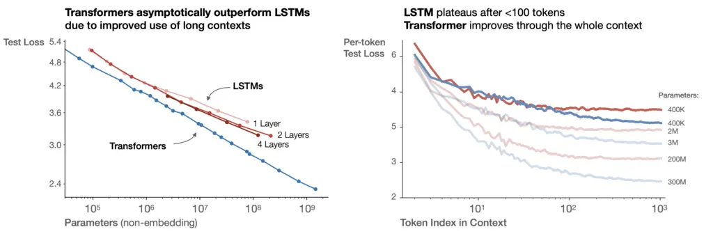
On the left plot, we see that the test loss of Transformers asymptotically beat that of LSTMs.

On the right plot (red plots are for LSTM, blue plots for Transformers), we see that while LSTM and Transformer curves have lower per-token losses at all indices as the number of parameters increases, this trend plateaus for LSTMs beyond some token index, but continues to decay for Transformers. The per-token loss should decrease as the index increases since there is more context to constrain the possibilities of the next token.

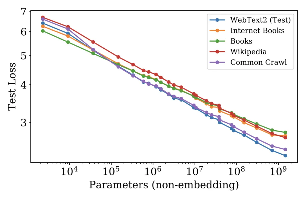
4. Generalization Among Data Distributions

The authors also verified that the scaling laws hold for different data distributions:

Most Glaring Deficiency

I thought the paper was generally very comprehensive and analyzed the scaling laws from many different dimensions. However, it could have gone a step further to distill the learnings from the results to provide concrete guidelines on how to choose \(N, C, D\) when training LLMs.

Conclusions for Future Work

Given a fixed compute budget, one can choose \(N, D\) appropriately to achieve a desired loss.

While the paper provided empirical evidence for the scaling laws, there is not yet any theoretical understanding of why this is the case, which would be an interesting line of future research.