Research Sprint Day 3 - Seed Noise and Transformer Baselines
Training transformer baselines at 30M, 60M, and 125M to measure how much random seed alone moves final validation loss. Pooled seed noise comes out at 0.003 nats, which sets the minimum effect size for every architecture comparison to follow

I’m doing a 30 day research sprint on linear attention. Today is day 3. All code lives in this repository.
Yesterday, we performed some performance benchmarking to get a sense of what MFU to expect across various model sizes between both attention and GDN.
Today, we investigate seed noise in transformer models (before proceeding with GDN subsequently), so we know what’s the minimum detectable difference of an effect before we can claim an improvement.
Setup
Data
All runs train on FineWeb-Edu, the educational-quality filtered subset of FineWeb, using its sample-10BT split. The text is tokenized with the GPT-2 tokenizer and written in the llm.c shard format as 16 shards of 100M tokens each. Shard 0 is held out for validation and never trained on; shards 1 to 15 (1.5B tokens) are the training pool. The largest budget today is 1.2B tokens, so no run sees a token twice.
Training examples are aligned windows of $T = 1024$ tokens cut from the training shards. The set of windows is fixed across runs; what the seed changes is the initialization and the order in which those windows are visited.
The GPT-2 tokenizer has 50,257 tokens, which we pad to $V = 50{,}304$ (a multiple of 64) for the embedding and LM head. Note that yesterday’s throughput benchmarks used $V = 32{,}000$, chosen so that the LM head would not dominate the FLOPs of the smaller models during benchmarking. Today’s vocabulary is the real one, so the day 2 throughput numbers need a correction before they can be used for time estimates (see Predictions below).
Models
We’ll be training at 3 different model sizes (excluding the 250M as it would take prohibitively long on the compute I have). The models will be undertrained (only ~10x) due to compute limitations.
| Size | $d$ | $L$ | Heads | Body params | Embedding + head | Budget $D$ |
|---|---|---|---|---|---|---|
| 30M | 512 | 10 | 8 | 34.1M | $2 \times 25.8$M | 300M |
| 60M | 768 | 9 | 12 | 63.7M | $2 \times 38.6$M | 600M |
| 125M | 768 | 18 | 12 | 127.4M | $2 \times 38.6$M | 1.2B |
Benchmarked numbers from day 2:
| Size | tok/s | MFU % | BW % |
|---|---|---|---|
| 30M | 77,546 | 27.2 | 21.0 |
| 60M | 59,511 | 35.7 | 22.4 |
| 125M | 32,926 | 34.4 | 24.0 |
Training setup:
| Setting | Value |
|---|---|
| Optimizer | AdamW, $\beta = (0.9, 0.95)$, weight decay 0.1 on matrices, 0 on norm gains, fused |
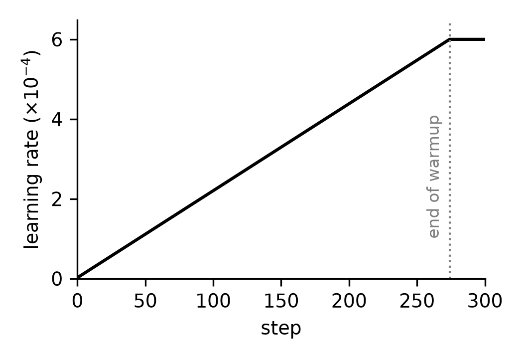
| Learning rate | peak $6 \times 10^{-4}$, 3% linear warmup, cosine to $0.1 \times$ peak |
| Batch | $B = 32$ windows of $T = 1024$ tokens; $32{,}768$ tokens per step |
| Precision | bf16 autocast, fp32 master weights; no torch.compile |
| Attention | PyTorch’s built-in FlashAttention kernel (F.scaled_dot_product_attention restricted to SDPBackend.FLASH_ATTENTION) |
| Clipping | global gradient norm 1.0 |
| Evaluation | every 5% of $S$ on 4096 windows; final on $16{,}384$ windows of shard 0 |
| Checkpoints | weights (bf16) every 10% of $S$; full state for resuming at the same points |
| Seeds | 0 and 1; the seed sets the initialization and the window order, not the window set |
Predictions
Estimates for training time
We did benchmarking previously at a smaller vocab size, so we will scale throughput by a fraction proportionate to the change in vocab size to model size.
Let $D$ be the token budget, $\hat{v}$ the throughput benchmarked on day 2, and $c$ the correction factor that discounts that throughput for the larger vocabulary. The expected wall-clock time of a single run is then
\[t_{\text{run}} = \frac{D}{c\,\hat{v}},\]with $c = 0.88, 0.90, 0.92$ for 30M, 60M, and 125M respectively. the penalty shrinks with model size because the LM head is a smaller share of total FLOPs in the larger models. This gives:
| Size | $D$ | $\hat{v}$ (tok/s) | $c$ | $c\,\hat{v}$ (tok/s) | $t_{\text{run}}$ | Both seeds |
|---|---|---|---|---|---|---|
| 30M | 300M | 77,546 | 0.88 | 68,240 | 1.2 h | 2.4 h |
| 60M | 600M | 59,511 | 0.90 | 53,560 | 3.1 h | 6.2 h |
| 125M | 1.2B | 32,926 | 0.92 | 30,292 | 11.0 h | 22.0 h |
So all six runs (three sizes $\times$ two seeds) should take roughly 31 GPU-hours, excluding evaluation and checkpointing overhead.
Peak memory
The throughput measurement at 30M yesterday peaked at 9.3 GB with V=32_000.
Let’s estimate how much it would increase at today’s V=50_304.
The difference in memory usage would come from: fp32 weights, fp32 optimizer states for Adam, fp32 gradients, and logits.
For each of the embedding and unembedding matrices, model state would account for $4 + 4 + 4 + 4 = 16$ bytes per parameter. The total increase in parameters is $(V_{new} - V_{old}) \times d = (50,304 - 32,000) \times 512 = 9.37M$, so for a total of $9.37M \times 16 \text{ bytes/param} = 150MB $. Including both embedding and unembedding we get $300MB$.
The difference in activation is a bit more involved, as it requires knowledge of implementation details. fla TransformerForCausalLM defaults to fuse_cross_entropy=True, so it never ends up materializing the full $(B, T, V)$ tensor at fp32 while computing cross entropy in both the forward and backward. This leaves just a single $(B, T, V)$ logit tensor in bf16, which creates a difference of $B \times T \times (V_{new} - V_{old}) \times 2 = 32 \times 1024 \times (50,304 - 32,000) \times 2 = 1.2GB$.
The net difference we would expect to see is hence an increase in $300MB + 1.2GB = 1.5GB$ of memory usage, for a total of $9.3GB + 1.5GB = 10.8GB$.
Final validation loss
We borrow the constants from Chinchilla scaling laws. The constants will be off in some ways since we are using a different tokenizer.
\[L(N, D) = E + \frac{A}{N^{\alpha}} + \frac{B}{D^{\beta}}, \quad E = 1.69,\; A = 406.4,\; B = 410.7,\; \alpha = 0.34,\; \beta = 0.28\]The Chinchilla paper used total parameters for $N$ (whereas the Kaplan paper used non-embedding parameters only). We’ll do it for both total parameters and non-embedding parameters for the sake of comparison:
| Size | Budget $D$ | $N$ (total) | $L(N,D)$ total | $N$ (non-emb) | $L(N,D)$ non-emb | Gap |
|---|---|---|---|---|---|---|
| 30M | 300M | 85.7M | 4.24 | 34.1M | 4.54 | 0.30 |
| 60M | 600M | 140.9M | 3.81 | 63.7M | 4.02 | 0.21 |
| 125M | 1.2B | 204.6M | 3.48 | 127.4M | 3.58 | 0.11 |
Pooled seed noise
Inter-run standard deviation of 0.01 nats? I feel woefully uncalibrated.
Does seed noise shrink with larger models?
Prediction: yes.
However, at 2 seeds at each configuration, we’ll see whether we can observe this effect…
Non-determinism floor
Beyond seed noise, we also saw that the GPU can introduce non-determinism. In particular, the FlashAttention backward is non-deterministic by default.
Guess: 0.01 in same-seed max absolute difference in loss after 300 steps of training.
Validating setup
Validation loss on untrained 30M model (d=512) is 10.9294.
The standard analysis would claim that each head logit has mean zero, and hence cross entropy loss for each token simplifies to $\log \sum_j e^{z_j} - z_y = \log V - 0 = \log V $. At vocab size 50304, this gives $\ln 50304 = 10.826$, which is slightly smaller than what we saw.
Of course, the logits are only 0 in expectation, so this analysis is a rough approximation that doesn’t hold up in practice, evidenced by the gap.
We will show that in fact, the initial loss is close to \(\log V + s^2d/2.\)
In fla, the LM head is Gaussian initialized from $\mathcal{N}(0, s^2)$ with $s=0.02$. Each $z_i$ is the dot product between the activations $h$ from the previous layer, and its corresponding $d$ weights $w_i$. So this is the sum of scaled Gaussians (where $w_{ik}$ is scaled by by $h_k$), which gives that
How do we figure out what $\sum_k h_k^2$ is? Fortunately, we have a RMSNorm layer before the output head, so in fact $\sum_k h_k^2 = d$, and
\[z_i \sim \mathcal{N} \left(0, s^2d \right).\]Write $v=s^2d$. Now to understand the distribution of $e^{z_i}$, we show that $\mathbb{E}[e^Z] = e^{v/2}$ for $Z \sim \mathcal{N}(0, v)$:
\[\mathbb{E}[e^Z] = \int_{-\infty}^{\infty} \frac{1}{\sqrt{v}\sqrt{2\pi}} \exp\left(-\frac{z^2}{2v}\right) \exp(z) \, dz\] \[= \int_{-\infty}^{\infty} \frac{1}{\sqrt{2\pi v}} \exp\left(z - \frac{z^2}{2v}\right) dz\]By completing the square:
\[z - \frac{z^2}{2v} = -\frac{(z - v)^2}{2v} + \frac{v}{2}\]Substituting back:
\[= \exp\left(\frac{v}{2}\right) \int_{-\infty}^{\infty} \frac{1}{\sqrt{2\pi v}} \exp\left(-\frac{(z - v)^2}{2v}\right) dz\]The integrand is the probability density function (pdf) of $\mathcal{N}(v, v)$, and so the integral must equal 1.
\[= \exp\left(\frac{v}{2}\right)\]One can then make a claim that due to the small variance of the mean (over large $V$) $\mathbb{E} \left[ \log \sum_j e^{z_j} \right] \approx \log \sum_j \mathbb{E} \left[ e^{z_j} \right]$. The full proof is long and ugly and omitted for brevity, but main idea is to compute variance of the mean as eps and perform first-order Taylor expansion around log with this eps error.
This finally gives loss for each token as
$\log \sum_j e^{z_j} - z_y = \log (V \exp(s^2d/2)) - z_y = \log V + s^2d/2 - z_y $, and by taking expectations $z_y=0$, so the final loss is about
\[\log V + s^2d/2,\]which gives $10.825 + 0.02^2 \times 512 / 2 = 10.928$, very close to the actual value that we observed of 10.929.
Experiments
Results:
| Run | Size | Seed | Steps | Tokens | Val loss @ step 0 | Final val loss | Train tok/s | Peak mem (GB) | Hours |
|---|---|---|---|---|---|---|---|---|---|
| attn_30M_s0 | 30M | 0 | 9,155 | 300M | 10.929 | 3.7418 | 71,733 | 11.1 | 0.53$^*$ |
| attn_30M_s1 | 30M | 1 | 9,155 | 300M | 10.932 | 3.7465 | 71,709 | 10.8 | 1.29 |
| attn_60M_s0 | 60M | 0 | 18,310 | 600M | 11.011 | 3.4870 | 54,014 | 13.4 | 3.26 |
| attn_60M_s1 | 60M | 1 | 18,310 | 600M | 10.957 | 3.4886 | 53,809 | 13.4 | 3.28 |
| attn_125M_s0 | 125M | 0 | 36,621 | 1.2B | 10.980 | 3.2558 | 30,908 | 23.1 | 2.26$^*$ |
| attn_125M_s1 | 125M | 1 | 36,621 | 1.2B | 10.964 | 3.2616 | 30,637 | 22.2 | 11.31 |
$*$: wall-clock of the final segment only. These runs died from thermal shutdown partway through and were resumed from a checkpoint, and the hours field does not add up the time across segments.
Measuring seed noise
Under the assumption of homoscedasticity, i.e that seed noise doesn’t vary across model sizes (this is not true in practice - there’s generally less noise in larger models), we can pool the observations across seeds across model sizes to measure seed noise with pooled variance:
\[\hat{s}^2_{\text{pooled}} = \frac{\sum_{i \in \text{sizes}} \sum_{j \in \text{seeds}} \left( x_{ij} - \bar{x}_i \right)^2}{\sum_{i} \left( n_i - 1 \right)}\]Here $n_i$ is the number of seeds at a particular model size, and so $n_i- 1$ represents the degrees of freedom $\nu$.
Computing seed noise of final validation loss at each level, and pooled:
| Size | Loss s0 | Loss s1 | $\hat{s}$ (nats) | $\nu$ | 80% range for $\sigma$ |
|---|---|---|---|---|---|
| 30M | 3.7418 | 3.7465 | 0.0033 | 1 | [0.0020, 0.0263] |
| 60M | 3.4870 | 3.4886 | 0.0012 | 1 | [0.0007, 0.0095] |
| 125M | 3.2558 | 3.2616 | 0.0041 | 1 | [0.0025, 0.0325] |
| Pooled | 0.0031 | 3 | [0.0022, 0.0070] |
The pooled seed noise of 0.003 was within a magnitude off from my prediction of 0.01. My previous prediction that seed noise decreases with model size does not seem resolvable with the current $\nu=1$.
Verifying predictions: non-determinism floor
I ran the 30M model on seed 0 for 300 steps twice:
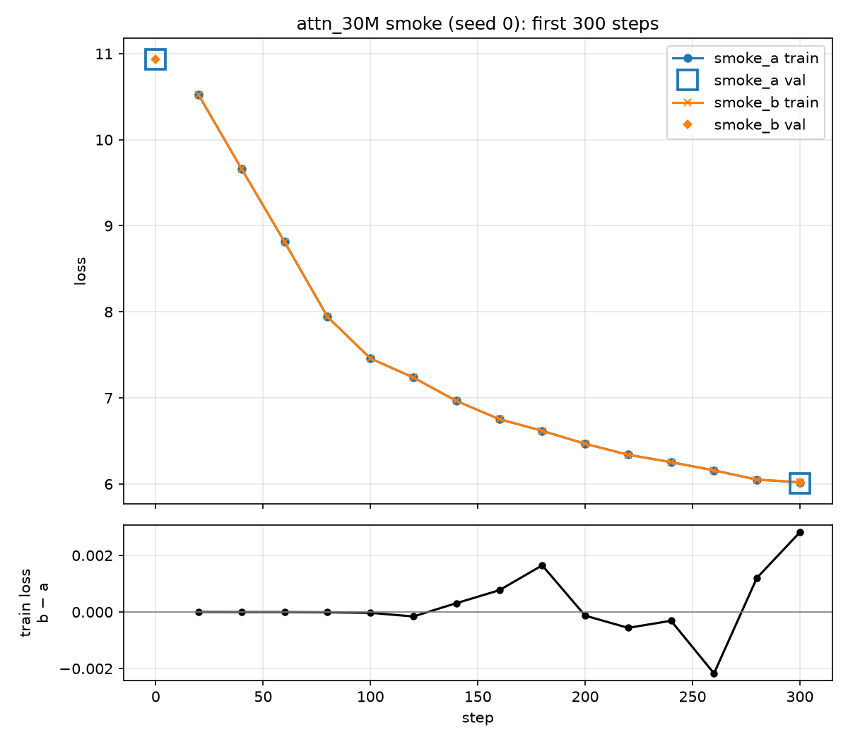
The drift increases over time, likely due to increasing LR over LR schedule warmup:
The maximum drift over these step was around 0.002, smaller than my guess of 0.01.
It would also be interesting to investigate the extent of drift over the full course of training.
Verifying predictions: initial loss
The prediction above depends on the model width through the $s^2 d / 2$ term, so the two widths get different predictions:
| $d$ | $\ln V$ | $s^2 d / 2$ | Predicted initial loss |
|---|---|---|---|
| 512 | 10.826 | 0.102 | 10.928 |
| 768 | 10.826 | 0.154 | 10.979 |
Against the measured validation loss at step 0:
| Run | $d$ | Predicted | Measured | Residual |
|---|---|---|---|---|
| attn_30M_s0 | 512 | 10.928 | 10.929 | $+0.001$ |
| attn_30M_s1 | 512 | 10.928 | 10.932 | $+0.004$ |
| attn_60M_s0 | 768 | 10.979 | 11.011 | $+0.032$ |
| attn_60M_s1 | 768 | 10.979 | 10.957 | $-0.022$ |
| attn_125M_s0 | 768 | 10.979 | 10.980 | $+0.001$ |
| attn_125M_s1 | 768 | 10.979 | 10.964 | $-0.015$ |
The predictions are pretty close to what we observed, and the residuals have no consistent sign, so there is no bias.
Verifying predictions: peak memory
We previously predicted $10.8GB$ peak memory usage at 30M. Looking at our logs, peak_mem_GB was $10.78GB$. Pretty spot on!
Verifying predictions: training time
| Size | $t_{\text{pred}}$ | $t_{\text{actual}}$, seed 0 | $t_{\text{actual}}$, seed 1 |
|---|---|---|---|
| 30M | 1.2 h | 0.53 h$^*$ | 1.29 h |
| 60M | 3.1 h | 3.26 h | 3.28 h |
| 125M | 11.0 h | 2.26 h$^*$ | 11.31 h |
$*$: wall-clock of the final segment only. These runs died from thermal shutdown partway through and were resumed from a checkpoint, and the hours field does not add up the time across segments.
Verifying predictions: final loss
| Size | $N$ (total) | $L(N,D)$ total | $N$ (non-emb) | $L(N,D)$ non-emb | Actual s0 | Actual s1 | Actual avg |
|---|---|---|---|---|---|---|---|
| 30M | 85.7M | 4.24 | 34.1M | 4.54 | 3.7418 | 3.7465 | 3.7442 |
| 60M | 140.9M | 3.81 | 63.7M | 4.02 | 3.4870 | 3.4886 | 3.4878 |
| 125M | 204.6M | 3.48 | 127.4M | 3.58 | 3.2558 | 3.2616 | 3.2587 |
Actual final loss was less than predictions with Chinchilla constants:
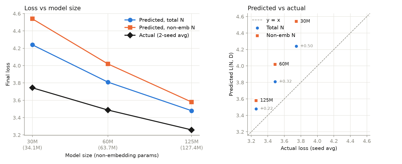
Some possible reasons for the divergence:
- We used FineWeb-Edu (high-quality educational dataset) as our dataset, which is a lower-entropy dataset than web data in general
- We’re using a GPT-2 tokenizer with vocab size 50,304 instead of Gopher’s 32k. Although to first order, a larger vocab size should result in higher loss. We can use bits per byte to remove the tokenizer confounder.
- Chinchilla models are fitted with at least 5B tokens of data (our max is 1.2B), so we may be in a regime of extrapolation error
Loss
A Confusion about Trends
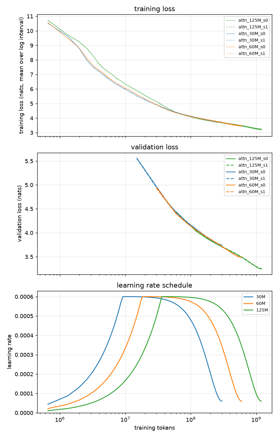
When I saw these plots, I initially felt quite confused due to how close all the lines were. It seemed to imply loss was a function of dataset size and didn’t seem to be affected by model size. Scaling law theory would’ve predicted that they should be a constant size apart.
Computing the $AN^{-\alpha}$ term for each model size:
| Size | $N$ (total) | $A N^{-\alpha}$ |
|---|---|---|
| 30M | 85.7M | 0.816 |
| 60M | 140.9M | 0.689 |
| 125M | 204.6M | 0.607 |
So the maximum difference here between the smallest and largest model is 0.2 nats, which would’ve been visible on the plot.
However, after thinking about it further, scaling laws only tell us what happens at the end of training (i.e with full WSD schedules), and the intermediate states are not really comparable due to differences in schedule.
Another confounder is that the models are intentionally undertrained due to compute limitations. It is possible that we have yet to train on enough tokens for the smaller models to show the limitations of model capacity.
Next steps
We have estimated seed stddev at 3e-3 nats and have established our transformer baselines. We will subsequently proceed to training GDNs.
If I found more compute, performing scaling laws analysis to ensure I could actually replicate the theory would also be interesting.