Research Sprint Day 2 - Benchmarking
Benchmarking attention against Gated DeltaNet from 30M to 250M, where at this scale GDN costs 1.5× the time for roughly the same FLOPs
I’m doing a 30 day research sprint on linear attention. Today is day 2. All code lives in this repository.
In day 1, we established that the fla GDN kernel is sound numerically on our hardware. Today, we perform some performance benchmarking to get a sense of what MFU to expect across various model sizes between both attention and GDN.
Rooflines
Let’s benchmark our hardware to see how it stacks up with the advertised numbers.
GB10 theoretical: bf16 FLOPS: 118.8 TFLOP/s, memory bandwidth: 273 GB/s
FLOPs is benchmarked with $(8192, 8192) \times (8192, 8192)$ dense matmuls. Bandwidth is benchmarked by copying a 2GB tensor.
| Quantity | Measured | Theoretical peak | Fraction of peak |
|---|---|---|---|
| bf16 matmul throughput | 95.45 TFLOP/s | 118.8 TFLOP/s | 80.3% |
| Memory bandwidth (copy) | 222.37 GB/s | 273.0 GB/s | 81.5% |
| Ridge point ($I^*$) | 429.25 FLOP/byte | 435.16 FLOP/byte | 98.6% |
The ridge point is the ratio between peak FLOPs and HBM, which is the threshold between where we go from memory-bound to compute-bound.
Attention Backends
I checked that all attention kernels supported on PyTorch ["FLASH_ATTENTION", "EFFICIENT_ATTENTION", "CUDNN_ATTENTION", "MATH"] runs on my hardware. This is so we can explicitly use a tiling kernel afterwards in our comparisons between attention and GDN (as opposed to the naive MATH kernel that materializes the entire attention matrix).
Let’s see which one is fastest, with B=32, T=1024, d_h=64, and causal masking, across various head counts H:
H= 8 FLASH_ATTENTION         5.07 ms
H= 8 EFFICIENT_ATTENTION     6.38 ms
H= 8 CUDNN_ATTENTION         5.52 ms
H=12 FLASH_ATTENTION         7.74 ms
H=12 EFFICIENT_ATTENTION     9.64 ms
H=12 CUDNN_ATTENTION         8.26 ms
H=16 FLASH_ATTENTION        10.23 ms
H=16 EFFICIENT_ATTENTION    12.52 ms
H=16 CUDNN_ATTENTION        11.16 ms
Looks like FLASH_ATTENTION won here.
Building some intuition between attention and GDN
GDN update: \(\mathbf{S}_t = \mathbf{S}_{t-1}\left(\alpha_t(\mathbf{I} - \beta_t \boldsymbol{k}_t \boldsymbol{k}_t^\mathsf{T})\right) + \beta_t \boldsymbol{v}_t \boldsymbol{k}_t^\mathsf{T}\)
Also laying out the pseudocode, which makes it clearer what we are referring to when doing resource accounting in subsequent sections:
# x: (B, T, D)

# ---- 1. projections ----
q = q_proj(x)          # (B, T, H*d_k)
k = k_proj(x)          # (B, T, H*d_k)
v = v_proj(x)          # (B, T, H*d_v)

# ---- 2. short causal depthwise conv (kernel 4) + SiLU, per path ----
q = silu(shortconv_q(q))    # (B, T, H*d_k)
k = silu(shortconv_k(k))    # (B, T, H*d_k)
v = silu(shortconv_v(v))    # (B, T, H*d_v)

# ---- 3. split heads ----
q = reshape(q, B, T, H, d_k)
k = reshape(k, B, T, H, d_k)
v = reshape(v, B, T, H, d_v)

# ---- 4. L2-normalise queries and keys along the last axis ----
q = q / ||q||_2      # each (B,T,H,·) row has unit norm
k = k / ||k||_2

# ---- 5. the two gates: one SCALAR per (token, head) ----
beta  = sigmoid(b_proj(x))                              # (B, T, H), in (0,1)
if allow_neg_eigval: beta = 2 * beta                    # in (0,2)

g = -exp(A_log) * softplus(a_proj(x) + dt_bias)         # (B, T, H), <= 0
alpha = exp(g)                                          # (B, T, H), in (0,1)
# A_log: (H,) learned;  dt_bias: (H,) learned
# g is kept in log space because the kernel accumulates cumulative decay
# as a cumsum of g rather than a product of alpha (numerically safer).

# ---- 6. the recurrence (this is the whole paper) ----
o = gated_delta_rule(q, k, v, alpha, beta)              # (B, T, H, d_v)

# ---- 7. output gate + norm + projection ----
z = reshape(g_proj(x), B, T, H, d_v)                    # (B, T, H, d_v)
o = RMSNorm(o) * silu(z)                                # normalise per head, then gate
o = o_proj(reshape(o, B, T, H*d_v))                     # (B, T, D)
Note that we have $H d_k = D$, $Hd_v = e_v D$, where $e_v$ is the value-dimension expansion ratio, i.e size of value and output head dim relative to query and key head dim.
State
In attention, we need to store the KV cache for all previous tokens. Total state size: $T \times n_{heads} \times (d_k + d_v)$.
GDN’s state has size $d_v \times d_k$ per head. So state is fixed at $n_{heads} \times d_k \times d_v$.
Setting $T \, n_{heads} (d_k + d_v) = n_{heads} \, d_k d_v$ gives a crossover point of
\[T^\star = \frac{d_k d_v}{d_k + d_v},\]Past $T^\star$, GDN’s state is smaller than attention’s, and the compression ratio $T/T^\star$ grows linearly with context.
FLOPs per token
Attention does $6 \cdot 4D^2$ FLOPs (for QKVO) in projections, and $6TD$ FLOPs for attention, for a total of $24D^2 + 6TD$ for each token across both forward and backward.
The GDN update can be written in a fused manner, where instead of having to compute two outer products if we just apply the update naively, we can trim it down to one:
\[\begin{aligned} S_t &= S_{t-1}\big(\alpha_t (I - \beta_t k_t k_t^{T})\big) + \beta_t v_t k_t^{T} \\ &= \alpha_t S_{t-1} - \alpha_t \beta_t S_{t-1} k_t k_t^{T} + \beta_t v_t k_t^{T} \\ &= \alpha_t S_{t-1} + \big(\beta_t v_t - \alpha_t \beta_t S_{t-1} k_t\big) k_t^{T} \quad \text{(fused)} \end{aligned}\]In the forward pass, across all heads:
- $S_{t-1} k_t$ costs $2 D d_v$
- Outer product costs $2 D d_v$
- $o_t = S_t q_t$ costs $2 D d_v$
- Total: $6 D d_v$
In addition, we have the QK projection of $2 \cdot 2D^2$, the value, gate, and output projections of $3 \cdot 2 e_v D^2$,
So in total the forward pass is $6Dd_v + 4D^2 + 6e_vD^2$. With a typical $e_v=2$, this simplifies to $6Dd_v + 16D^2$. Then overall it requires $48D^2 + 18Dd_v$.
So in summary:
- GDN: $48D^2 + 18Dd_v$
- Attention: $24D^2 + 6TD$
We see that the projection cost for GDN dominates, and is double of that for attention.
Setting them equal and dividing by $6D$, we get the crossover sequence length where GDN becomes more efficient:
\[24D^2 + 6TD = 48D^2 + 18Dd_v \implies \boxed{T^\star = 4D + 3d_v}\]Experiments
We use the following model ladder, with batch size 32 and sequence length 1024:
| Size | Hidden size | Layers |
|---|---|---|
| 30M | 512 | 10 |
| 60M | 768 | 9 |
| 125M | 768 | 18 |
| 250M | 1024 | 20 |
Benchmark results
| mixer | size | $d$ | $L$ | body M | tok/s | µs/tok | peak GB | MFU % | impl. GB/s | BW % |
|---|---|---|---|---|---|---|---|---|---|---|
| attn | 30M | 512 | 10 | 34.1 | 77,546 | 12.9 | 9.3 | 27.2 | 46.7 | 21.0 |
| gdn | 30M | 512 | 10 | 39.5 | 51,475 | 19.4 | 12.8 | 18.7 | 24.4 | 11.0 |
| attn | 60M | 768 | 9 | 63.7 | 59,511 | 16.8 | 11.8 | 35.7 | 49.7 | 22.4 |
| gdn | 60M | 768 | 9 | 74.5 | 38,155 | 26.2 | 16.7 | 24.4 | 25.5 | 11.5 |
| attn | 125M | 768 | 18 | 127.4 | 32,926 | 30.4 | 20.6 | 34.4 | 53.4 | 24.0 |
| gdn | 125M | 768 | 18 | 149.1 | 20,308 | 49.2 | 30.3 | 22.8 | 26.1 | 11.7 |
| attn | 250M | 1024 | 20 | 256.9 | 20,570 | 48.6 | 30.6 | 40.2 | 50.7 | 22.8 |
| gdn | 250M | 1024 | 20 | 299.6 | 13,061 | 76.6 | 45.1 | 27.9 | 25.8 | 11.6 |
- body M refers to non-embedding parameters (including output head).
- peak GB is peak allocated device memory
- impl. GB/s is implied memory bandwidth, based on an estimate of how much bytes is moved per token for the model during training
- BW %: fraction of impl. GB/s of peak bandwidth
Observations
From our previous analysis, the crossover point where GDN becomes more efficient than attention at $T^\star = 4D + 3d_v$ is not met at our values of $T$, and hence GDN uses more compute and takes longer per token.
Attention MFU is much higher than GDN, which may be due to GDN utilizing many elementwise ops (L2 norm on Q/k, sigmoids for $\beta$, softplus for $\alpha$, SiLU after convolutions, etc) which hasn’t been torch compiled.
Chinchilla optimal training times
If we are to train the GDN Chinchilla-optimal (20 tokens/param), the tok/s readings from the benchmark would imply the following time to train:
| size | $N$ (body) | tokens | time | $N$ (total) | tokens | time |
|---|---|---|---|---|---|---|
| 30M | 39.5M | 0.79B | 4.3 h | 72.2M | 1.44B | 7.8 h |
| 60M | 74.5M | 1.49B | 10.9 h | 123.7M | 2.47B | 18.0 h |
| 125M | 149.1M | 2.98B | 40.8 h | 198.2M | 3.97B | 54.2 h |
| 250M | 299.6M | 5.99B | 127 h (5.3 d) | 365.2M | 7.30B | 155 h (6.5 d) |
This seems pretty sad for iteration speed. We may have to either undertrain it, or find ways to acquire more compute.
tokens/s comparison
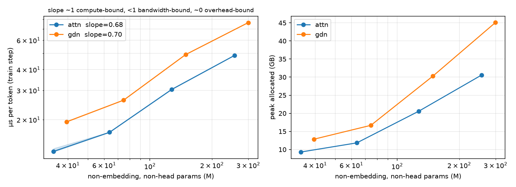
In the left plot, the GDN and attention lines are almost parallel of each other in the plot above, which in the log-log plot implies they are a constant ratio apart.
Since the gap is not size-independent, it is some overhead that scales with the size of the model, which is consistent with overhead from elementwise operations.
Arithmetic intensity vs observed
In the previous table, we also saw that neither MFU nor bandwidth was being saturated. Let’s look at the arithmetic intensity for each mixer across the model ladder:
| mixer | size | $F$ MFLOP/tok | $B$ kB/tok | $I$ = F/B | $I/I^*$ | MFU % | BW % |
|---|---|---|---|---|---|---|---|
| attn | 30M | 334 | 602 | 555 | 1.29 | 27.2 | 21.0 |
| gdn | 30M | 347 | 474 | 731 | 1.70 | 18.7 | 11.0 |
| attn | 60M | 572 | 836 | 684 | 1.59 | 35.7 | 22.4 |
| gdn | 60M | 611 | 667 | 915 | 2.13 | 24.4 | 11.5 |
| attn | 125M | 997 | 1621 | 615 | 1.43 | 34.4 | 24.0 |
| gdn | 125M | 1074 | 1284 | 836 | 1.95 | 22.8 | 11.7 |
| attn | 250M | 1864 | 2464 | 756 | 1.76 | 40.2 | 22.8 |
| gdn | 250M | 2041 | 1976 | 1033 | 2.41 | 27.9 | 11.6 |
All of them exceed the ridge point, but MFU and BW are both far from their ceiling.
GDN takes longer despite being similar in FLOPs
| size | FLOP ratio (gdn/attn) | time ratio (µs/tok) | |—|—:|—:| | 30M | 1.04 | 1.50 | | 60M | 1.07 | 1.56 | | 125M | 1.08 | 1.62 | | 250M | 1.09 | 1.58 |
Future work
- Sweep $T$ across both intermixers at the same size
-
torch.compilemight help GDN decently