A Markov chain that is aperiodic and irreducible will eventually converge to a stationary distribution. This is widely used in many applications in machine learning, such as in Markov Chain Monte Carlo (MCMC) methods, where random walks on Markov chains are used to obtain a good estimate of the log likelihood of the partition function of a model, which is hard to compute directly as it is #P-hard (this is even harder than NP-hard). However, one major issue is that it is unclear how many steps we should take before we are guaranteed that the Markov chain has converged to the true stationary distribution. In this post, we will see how the spectral gap of the transition matrix of the Markov Chain relates to its mixing time.

Mixing Times

Our goal is to try to develop methods to understand how long it takes to approximate the stationary distribution $π$ of a Markov Chain. Our goal is to eventually show that the mixing time is in $O (\frac{\log (n)}{1 - β})$ , where $β$ is the second largest eigenvalue of the transition matrix of the Markov Chain.

Aside: Coupling

Coupling is one general technique that allows us to bound how long it takes for a Markov Chain to converge to its stationary distribution based. It is based on having two copies of the original Markov Chain running simultaneously, with one being at stationarity, and showing how they can be made to coincide (i.e have bounded variation distance) after some time (known as the coupling time).

We will not discuss coupling in this post, but will instead develop how spectral gaps can be used, as this is more useful for other concepts.

The Spectral Gap Method

The main idea of the Spectral Gap method is that the mixing time is bounded by the inverse of the spectral gap, which is the difference between the largest and second largest eigenvalues of the transition matrix.

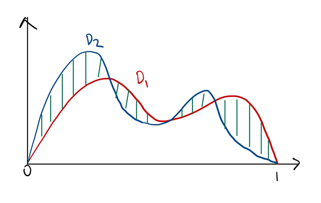
Before we can talk about one distribution approximating another, we need to first introduce what closeness between two distributions means The formulation that we will use is via the Total Variation Distance.

Definition (Total Variation Distance)

Let

D_{1}, D_{2}

be distributions on

Ω

. Then

\begin{aligned} (1) & ‖ D_{1} - D_{2} ‖_{T V} = & \frac{1}{2} \sum_{ω \in Ω} | D_{1} (ω) - D_{2} (ω) | \\ (2) & = & max_{A \subseteq Ω} \sum_{ω \in A} D_{1} (ω) - \sum_{ω \in A} D_{2} (ω) . \end{aligned}

The equality between the two lines can be observed from the fact that

\begin{array}{r} (3) & max_{A \subseteq Ω} \sum_{ω \in A} D_{1} (ω) - \sum_{ω \in A} D_{2} (ω) = max_{B \subseteq Ω} \sum_{ω \in B} D_{2} (ω) - \sum_{ω \in B} D_{1} (ω), \end{array}

since both $D_{1}, D_{2}$ are probability distributions and integrate to 1. See Figure 1 for an illustration.

*Figure 1.* Total Variation distance between some sample $D_{1}, D_{2}$ illustrated by the sum of the shaded green regions.

Intuition for Mixing Times

We consider how long it takes to converge on some special graphs to build up intuition.

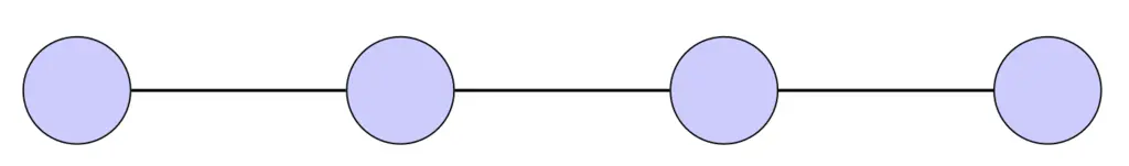
Random Walks on Path Graphs

The path graph is a line graph on $n$ vertices. We claim that the mixing time of the path graph is at least $n$ : this is because it takes at least $n$ steps to even reach the rightmost vertex from the leftmost vertex.

Random Walks on the Complete Graph

The complete graph $K_{n}$ on $n$ vertices is one where each vertex has an edge to every other vertex.

This only takes 1 step to mix, since after a single step we can reach any vertex.

*Figure 3.* The complete graph, $K_{6}$ .

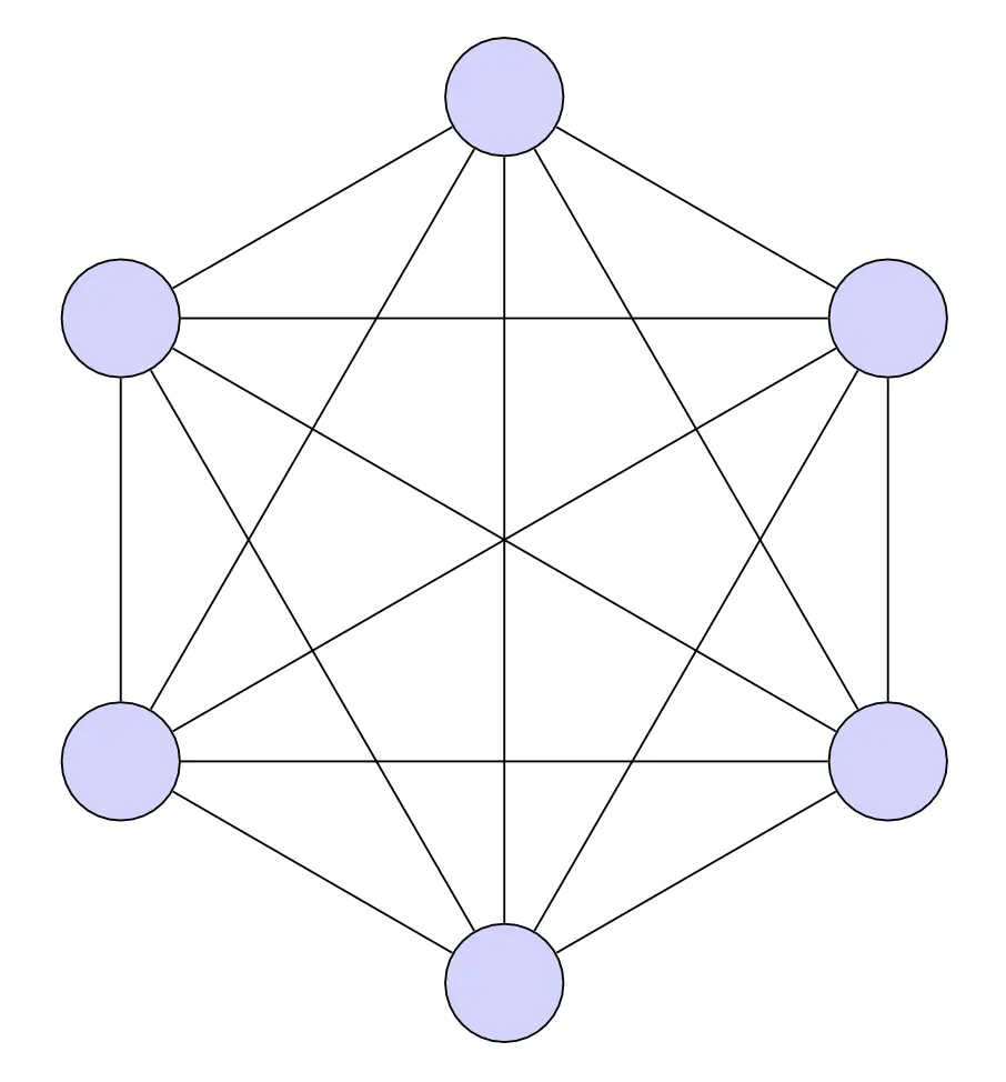
This short analysis tells us that if our graph looks like a line graph then we should expect poor mixing times; whereas if it looks more like a complete graph then we can expect the opposite.

Mixing Times

We now formally introduce the concept of mixing times.

Definition (Mixing Time)

Let

{X_{t}}

be a finite, irreducible, aperiodic Markov Chain,

π

be the stationary distribution, and

T

to be the transition matrix. Then define

\begin{array}{r} (4) & Δ (t) = max_{ω \in Ω} ‖ π - T_{ω}^{t} ‖_{T V}, \end{array}

where

T_{ω}^{t}

is the distribution of

X_{t}

given

X_{o} = ω

. In words,

Δ (t)

is the maximum time to converge to stationary distribution over all the starting points, where convergence is defined on total variation distance. Then the mixing time

τ_{mix}

is defined to be the smallest

t

such that

Δ (t) \leq \frac{1}{4}

We claim that the choice of $\frac{1}{4}$ in defining $τ_{mix}$ does not matter.

Proposition (Constants Don't Matter)

The choice of constant

\frac{1}{4}

does not matter. This is because for all

c \geq 1

Δ (c \cdot τ_{mix}) \leq \frac{1}{4^{c}}

. In other words, we can increase the mixing time by a linear amount to get an exponential decrease in total variation distance.

To bound mixing times, we consider random walks on undirected, regular graphs $G$ . The same analysis can be extended to directed, weighted, irregular graphs, but it causes the notation to become more cumbersome and distracts from the key ideas.

Consider random walks on an undirected, regular graph $G (V, E)$ , $| V | = n$ . Define the transition matrix $T$ of the graph to be

\begin{array}{r} (5) & T_{i j} = {\begin{cases} \frac{1}{\deg (j)} & if j \sim i \\ 0 & otherwise \end{cases} \end{array}

where $j \sim i$ means that $j$ shares an edge with $i$ .

The stationary distribution for $T$ is given by

\begin{array}{r} (6) & π = (\frac{\deg (1)}{2 | E |}, \dots, \frac{\deg (n)}{2 | E |}) . \end{array}

This can be seen from the following:

\begin{aligned} (7) & (T π)_{i} & = \sum_{j \in [n]} \frac{\deg (j)}{2 | E |} 1 \begin{array}{ll} {\begin{cases} \frac{1}{\deg (j)} & if j \sim i, \\ 0 & otherwise. \end{cases} \end{array}} \\ (8) & = \sum_{j \sim i} \frac{\deg (j)}{2 | E |} \frac{1}{\deg (j)} \\ (9) & = \frac{\deg (i)}{2 | E |} . \end{aligned}

If $G$ is $d$ -regular, then

\begin{array}{r} (10) & T = \frac{1}{d} \cdot A, \end{array}

where $A$ is the adjacency matrix of the graph.

Spectral Graph Theory

Spectral graph theory is the study of how the eigenvalues and eigenvectors of the matrix of a graph reveals certain properties about the graph, for instance, how well-connected it is.

Lemma (Lemma 1: Properties of the Adjacency Matrix of a

d

-regular Graph)

Let

T = \frac{1}{d} A

. Let

λ_{1} \geq λ_{2} \geq \dots \geq λ_{n}

to be the eigenvalues of

T

. Then the following properties hold:

$| λ_{i} | \leq 1$ for all $i$ , and $λ_{1} = 1$
$λ_{2} < 1$ if and only if $G$ is connected
$λ_{n} > - 1$ if and only if $G$ does not have a bipartite connected component

We prove each of the claims in Lemma 1 in order.

Proof (Claim 1:

| λ_{i} | \leq 1

for all

i

, and

λ_{1} = 1

)

Choose any eigenvector

v

.
Let

v_{i}

be the maximum magnitude entry of

v

. Observe that

v

is an eigenvector of

T

only if

T v = λ v

for some

λ

. Then

\begin{aligned} (11) & λ v_{i} & = (T v)_{i} \\ (12) & = \sum_{j \in N (i)} \frac{1}{d} \cdot v_{j} & (Multiplying i th row of T by v) \\ (13) & \leq | v_{i} | \end{aligned}

The last step comes from the fact that since each

| v_{j} | \leq | v_{i} |

, so at most we have

d \times \frac{1}{d} | v_{i} | = | v_{i} |

, recalling that

| N (i) | = d

since the graph is

d

-regular.

This shows that

| λ v_{i} | \leq | v_{i} |

for all

i

, and so

| λ | \leq 1

.

It remains to show that

λ_{1} = 1

. To see this, consider the vectors where all entries are 1, i.e

1

. Then

T \cdot 1 = 1

. So

1

is an eigenvector of

T

with eigenvalue 1.

Proof (Claim 2:

λ_{2} < 1

if and only if

G

is connected.)

(⟸)

Suppose that

G

is disconnected, we show that its second largest eigenvalue

λ_{2}

is 1.

WLOG, assume that the graph has two distinct connected components; the proof easily extends to having more components.
Let

S_{1}, S_{2}

be connected components of

G

. Recall that the connected components of

G

are the equivalence class of components where in each component, all vertices are reachable from any other vertex.

Define

v^{1}, v^{2}

via

\begin{array}{r} v_{i}^{1} = {\begin{cases} 1 & if i \in S_{1}, \\ 0 & otherwise, \end{cases} \\ v_{i}^{2} = {\begin{cases} 1 & if i \in S_{2}, \\ 0 & otherwise. \end{cases} \end{array}

Then

\begin{aligned} (14) & (T \cdot v^{1})_{i} & = \sum_{j \in N (i)} \frac{1}{d} v_{j}^{1} & (multiplying row i of T by v^{1}) \\ (15) & = \sum_{j \in N (i)} \frac{1}{d} 1 {j \in S_{1}} \\ (16) & = {\begin{cases} 1 & if i \in S_{1}, \\ 0 & otherwise. \end{cases} \end{aligned}

This shows that

T \cdot v^{1} = v^{1}

. Similarly, we can perform the same sequence of steps to derive that

T \cdot v^{2} = v^{2}

.

We can show the same for

v^{2}

to get

T \cdot v^{2} = v^{2}

. which shows that

λ_{2} = 1

.
Since by our disconnected assumption

v^{1}, v^{2} \neq 1

, the all-ones eigenvector corresponding to eigenvalue

λ_{1}

, it means

λ_{2} = 1

.
This shows the backwards direction.

(⟹)

For the other direction, suppose that

G

is connected, we want to show that

λ_{2} < 1

.

We will show that for any eigenvector

v

with eigenvalue

1

, then it must be a scaling of

1

.

Let

v

be any eigenvector with eigenvalue

1

. Then let

v_{i}

be its maximum entry. From Equation

11

, we must have that

\begin{aligned} (17) & λ v_{i} & = v_{i} \\ (18) & = (T v)_{i} \\ (19) & = \sum_{j \in N (i)} \frac{1}{d} \cdot v_{j} \\ (20) & = v_{i} . \end{aligned}

But since

v_{i}

is the largest entry, it must be the case that

v_{j} = v_{i}

for all

j \sim i

. We then repeat this argument to observe that all the neighbors of each

j

must also take on the same value. Since the graph is connected,

v

is just the uniform vector, as desired.

Note that this lemma shows that if

G

is disconnected, then it has a spectral gap of 0.

Proof (Claim 3:

λ_{n} > - 1

if and only if

G

does not have a bipartite connected component)

(⟹)

We show the forward direction by contraposition.
Suppose that

G

has a bipartite component

S

. We want to show that

λ_{n} = - 1

.

Let

S = L \cup R

denote the two disjoint bipartite components.

Define vector

\begin{array}{r} (21) & v_{i} = {\begin{cases} 1 & if i \in L, \\ - 1 & if i \in R, \\ 0 & otherwise. \end{cases} \end{array}

Again we compute

T \cdot v

, and consider its

i

th entry:

\begin{aligned} (22) & {(T \cdot v)}_{i} & = \sum_{j \in N (i)} \frac{1}{d} v_{j} \\ (23) & = - v_{i}, \end{aligned}

since the signs of its neighbors

N (i)

are always the opposite of the sign of

v_{i}

by construction.

Since

T v = - v

, this shows that we have an eigenvector with eigenvalue

- 1

(⟸)

Now suppose that

T v = - v

, with the goal to show that the graph is bipartite.
Similarly as for the backwards direction of Claim 2, we can see that this can only hold on each element

v_{i}

if all the signs of the neighbors of

v_{i}

have the same magnitude but opposite sign of

v_{i}

. Then we can similarly expand this argument to the neighbors of its neighbors, which shows that the graph is bipartite.

This shows how we can gleam useful information about a graph just from its eigenvalues.

Recall how we previously showed that a unique stationary distribution exists if the graph is connected and not bipartite. Now we have another characterization of the same property, except in terms of the eigenvalues of its transition matrix:

Corollary (Corollary of the Fundamental Theorem)

T

is such that

λ_{2} < 1

λ_{n} > - 1

then the random walk has a unique stationary distribution which is uniform.

Our goal now is to formulate a robust version of this corollary, where we can bound the mixing time of approaching the stationary distribution.

Bounding the Mixing Time via the Spectral Gap

We define the spectral gap:

Definition (Spectral Gap)

Given

T

, define

\begin{array}{r} (24) & β = max {λ_{2}, | λ_{n} |} = max_{2 \leq i \leq n} | λ_{i} | . \end{array}

Then the spectral gap is given by

\begin{array}{r} (25) & spectral_gap (T) = 1 - β . \end{array}

We now finally introduce a lemma that shows that the mixing time is proportional to the inverse of the spectral gap multiplied by a log factor:

Lemma (Lemma 2: Mixing Time of Markov Chains)

Suppose

T = \frac{1}{d} A

. Then

\begin{array}{r} (26) & τ_{mix} (T) \leq O (\frac{\log (n)}{1 - β}) . \end{array}

This shows that if your spectral gap is bounded by a constant, your mixing time is in $O (\log (n))$ .

Exercise

Verify that the path graph indeed has a small spectral gap, since we previously established that it has a large mixing time. Similarly, check that the complete graph has a large spectral gap.

Proof

We now prove Lemma 2.

Let $T$ have eigenvalues $1 = λ_{1} \geq λ_{2} \geq \dots \geq λ_{n}$ with eigenvectors $v^{1}, v^{2}, \dots, v^{n}$ . Assume that the eigenvectors are scaled to be unit vectors.

Since this is a symmetric matrix, the eigenvectors are pairwise orthogonal.

We can perform an eigenvalue decomposition of $T$ in terms of its eigenvectors via $\begin{array}{r} (27) & T = \sum_{i} λ_{i} v_{i} v_{i}^{⊤} . \end{array}$

It follows from Equation $27$ that $\begin{array}{r} (28) & T^{k} = \sum_{i} λ_{i}^{k} v_{i} v_{i}^{⊤} . \end{array}$

Let $x \in [0, 1]^{n}$ be a probability vector of $G$ where all entries are non-negative and sum to 1. Think of $x$ as the start state of the Markov chain.

After $k$ steps, the state will be $T^{k} \cdot x$ .

We can re-write $x$ in terms of the orthogonal basis of the eigenvectors of $T$ , i.e $\begin{array}{r} (29) & x = \sum_{i} ⟨ x, v_{i} ⟩ \cdot v_{i} . \end{array}$ Write $a_{i} = ⟨ x, v_{i} ⟩$ to be the coefficients of each eigenvector $v_{i}$ .

$λ_{1} = 1$ , so $λ_{1}^{k} = 1$ . We also know that

\begin{array}{r} (30) & v^{1} = (\begin{array}{c} \frac{1}{\sqrt{n}} \\ ⋮ \\ \frac{1}{\sqrt{n}} \end{array}), \end{array}

since we previously showed that the all-ones vector is always an eigenvector with eigenvalue 1, where here it is re-scaled to have unit norm.

Then $\begin{aligned} (31) & T^{k} \cdot x & = \sum_{i} ⟨ x, v_{i} ⟩ \cdot λ_{i}^{k} \cdot v_{i} \\ (32) & = ⟨ x, v^{1} ⟩ \cdot v^{1} + \sum_{i \geq 2} ⟨ x, v_{i} ⟩ \cdot λ_{i}^{k} \cdot v_{i} \\ (33) & = \frac{1}{n} ⟨ x, 1 ⟩ \cdot 1 + \sum_{i \geq 2} ⟨ x, v_{i} ⟩ \cdot λ_{i}^{k} \cdot v_{i} \\ (34) & = (\begin{array}{c} \frac{1}{n} \\ ⋮ \\ \frac{1}{n} \end{array}) + \sum_{i \geq 2} ⟨ x, v_{i} ⟩ \cdot λ_{i}^{k} \cdot v_{i}, \end{aligned}$

where the last step follows from the fact that $x$ is a probability distribution and thus $x \cdot 1 = 1$ .

Rearranging and moving to work in the L2 (Euclidean) norm, we obtain

\begin{aligned} (35) & {| | T^{k} \cdot x - (\begin{array}{c} \frac{1}{n} \\ ⋮ \\ \frac{1}{n} \end{array}) | |}_{2} & = {| | \sum_{i = 2}^{n} ⟨ x, v_{i} ⟩ \cdot λ_{i}^{k} v_{i} | |}_{2} \\ (36) & = \sqrt{\sum_{i = 2}^{n} ⟨ x, v_{i} ⟩^{2} \cdot λ_{i}^{2 k} \cdot ‖ v_{i} ‖_{2}^{2}} \\ (37) & (def of L2 norm, x-terms cancel as e.v are pairwise orth) \\ (38) & = \sqrt{\sum_{i = 2}^{n} ⟨ x, v_{i} ⟩^{2} \cdot λ_{i}^{2 k}} \\ (39) & (v_{i} has unit norm) \\ (40) & \leq ‖ x ‖_{2} \cdot β^{k}, \end{aligned}

where the last step comes from the fact that $λ_{i} \leq β$ for all $i \geq 2$ since $β$ is the second-largest eigenvalue, and $\sum_{i = 1}^{n} ⟨ x, v_{i} ⟩^{2} = | x |_{2}^{2}$ .

Since $| x |_{2} \leq 1$ , we can simplify

\begin{aligned} (41) & {| | T^{k} \cdot x - (\begin{array}{c} \frac{1}{n} \\ ⋮ \\ \frac{1}{n} \end{array}) | |}_{2} & \leq β^{k} \\ (42) & = (1 - (1 - β))^{k} . \end{aligned}

However, what we really care about is the total variation distance, which is the quantity

\begin{array}{r} (43) & \frac{1}{2} {| | T^{k} \cdot x - (\begin{array}{c} \frac{1}{n} \\ ⋮ \\ \frac{1}{n} \end{array}) | |}_{T V} \\ (44) & = \frac{1}{2} {| | T^{k} \cdot x - (\begin{array}{c} \frac{1}{n} \\ ⋮ \\ \frac{1}{n} \end{array}) | |}_{1} . \end{array}

Recall that for any $n$ -dimensional vector $x$ , $| x |_{1} = \sqrt{n} | x |_{s}$ by Cauchy-Schwarz:

\begin{aligned} (45) & ‖ x ‖_{1} & = 1 \cdot x \\ (by Cauchy-Schwarz) & \leq ‖ 1 ‖_{2} ‖ x ‖_{2} \\ (46) & = \sqrt{n} ‖ x ‖_{2} . \end{aligned}

To relate the L2 distance to L1 distance, we can apply the above inequality to get $\begin{aligned} (47) & \frac{1}{2} {| | T^{k} \cdot x - (\begin{array}{c} \frac{1}{n} \\ ⋮ \\ \frac{1}{n} \end{array}) | |}_{1} & \leq \frac{1}{2} \sqrt{n} {| | T^{k} \cdot x - (\begin{array}{c} \frac{1}{n} \\ ⋮ \\ \frac{1}{n} \end{array}) | |}_{2} \\ (48) \\ (49) & \leq \frac{1}{2} \sqrt{n} β^{k} \\ (if k > O (\frac{\log n}{1 - β})) & \leq \frac{1}{4}, \end{aligned}$ as desired.

So we set $k \geq O (\frac{\log n}{1 - β})$ for the total variation distance to be less than 1/4.

We say that a Markov Chain is fast mixing if $τ_{mix} \leq \log^{O (1)} (n)$ .

Expander Graphs

Lemma 2 motivates the following definition of expander graphs:

Definition (Expander Graphs)

G

is a

(n, d, ϵ)

-expander graph if

G

is a

d

-regular graph and

T = \frac{1}{d} A

has spectral gap at least

ϵ

From what we have learnt so far, we know that an expander has to be well-connected in order to have a large spectral gap. Expander graphs can be used for derandomization, which helps to reduce the amount of random bits required for algorithms.