Neural Networks from Maximizing Rate Reduction

The quest for a new white box modeling paradigm

While we have witnessed empirical evidence of the success of deep learning, much of it is attributable to trial and error and not guided by underlying mathematical principles. I attended Yi Ma’s keynote on Pursuing the Nature of Intelligence at ICLR this year, which took on a statistical lens towards urging the community to view model training as learning to do compression.

I was especially struck by the novelty of some of his recent work on using coding rate reduction as a learning objective, and the remainder of this post will be a high-level overview of his paper ReduNet: ReduNet: A White-box Deep Network from the Principle of Maximizing Rate Reduction .

The paper tries to answer the question of how to develop a principled mathematical framework for better understanding and design of deep networks?

To this end, they noted that all predictable information is encoded as a distribution of low-dimensional supports observed in high-dimensional data space, and hence compression is the only inductive bias that our models need. They come up with a constructive modeling approach called ReduNet hat uses the principle of maximal coding rate reduction.

ReduNet

ReduNet is motivated by the following three desiderata for a model: that features of samples from the same (resp. different) class belong to the same (resp. different) low-dimensional linear subspace, and that variance of features within a class should be as large as possible as long as they stay uncorrelated from other classes for diversity. This will result in features that can be easily discriminated by a linear model.

How can we measure the “compactness” of a distribution of these latents to achieve the goals above? We can’t use cross entropy as we want something that doesn’t depend on the existence of class labels so we can do unsupervised learning. We also can’t use information-theoretic measures like entropy or information gain, because it is not always well-defined on all distributions (i.e diverges for Cauchy). In addition, we want something that we can actually compute tractably using a finite number of samples as an approximation.

To do this, they use the coding rate of the features, defined as the average number of bits needed to encode a set of learned representations $Z = [z^1, \cdots, z^m]$ with each $z^i \in \R^d$, each of which can be recovered up to some error $\epsilon$ via a codebook: $\mathcal{L}(\boldsymbol{Z}, \epsilon) \doteq\left(\frac{m+n}{2}\right) \log \operatorname{det}\left(\boldsymbol{I}+\frac{n}{m \epsilon^2} \boldsymbol{Z} \boldsymbol{Z}^*\right)$. If $m \gg n$ as is the case, then the average coding rate is

\[R(\boldsymbol{Z}, \epsilon) \doteq \frac{1}{2} \log \operatorname{det}\left(\boldsymbol{I}+\frac{n}{m \epsilon^2} \boldsymbol{Z} \boldsymbol{Z}^*\right)\]

We can similarly define the average coding rate for each class of the data, where $\mathbb{\Pi}^j$ encodes the probability of membership for class $j$:

\[R_c(\boldsymbol{Z}, \epsilon \mid \boldsymbol{\Pi}) \doteq \sum_{j=1}^k \frac{\operatorname{tr}\left(\boldsymbol{\Pi}^j\right)}{2 m} \log \operatorname{det}\left(\boldsymbol{I}+\frac{n}{\operatorname{tr}\left(\boldsymbol{\Pi}^j\right) \epsilon^2} \boldsymbol{Z} \boldsymbol{\Pi}^j \boldsymbol{Z}^*\right)\]

The point of defining $R$ and $R_c$ this way is that we want to maximize the coding rate over the entire dataset while minimizing the coding rate within each class, which encourages inter-class subspaces to be orthogonal. Furthermore, controlling for $\epsilon$ allows us to preserve intra-class diversity of features.

This gives us the following objective:

\[\max _{\boldsymbol{\theta}, \boldsymbol{\Pi}} \Delta R(\boldsymbol{Z}(\boldsymbol{\theta}), \boldsymbol{\Pi}, \epsilon)=R(\boldsymbol{Z}(\boldsymbol{\theta}), \epsilon)-R_c(\boldsymbol{Z}(\boldsymbol{\theta}), \epsilon \mid \boldsymbol{\Pi}), \quad$ s.t. $\left\|\boldsymbol{Z}^j(\boldsymbol{\theta})\right\|_F^2=m_j, \boldsymbol{\Pi} \in \Omega,\]

where the constraint is to ensure that feature sizes are normalized.

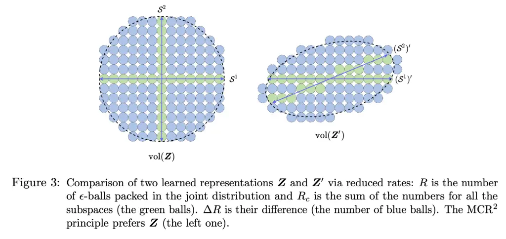
Intuitively, the picture looks like the below, where we try to maximize size of our codebook (i.e balls) to capture all the data whilst minimizing the codebook of each individual class:

Training

The neat thing about these networks is that we only have to train it layer by layer sequentially with just forward propagation (no backpropagation).

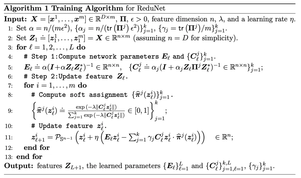
In plaintext, it works as follows:

Suppose we want to train a ReduNet with $L$ layers
Initialize our initial set of features to be the same as our data
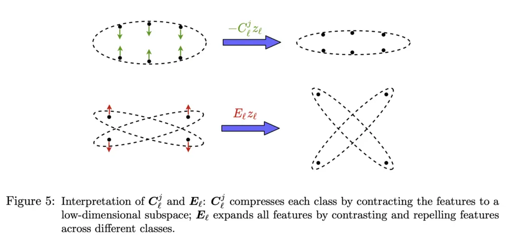
Compute our gradients $\bE_{\ell}$ for the $R$ term and $\bC^j_{\ell}$ for the $R_c$ term (note that this is just gradients for just layer $l$)
Compute soft assignments in feature space (I didn’t understand the requirement for this fully, but I think it stems from the need to support the unsupervised context when the true class labels aren’t known)
Output new features with the expression in line 6, normalized by projecting onto the unit sphere $\mathcal{P}$
Repeat for each subsequent layer

Geometrically, at each step the features across classes become increasingly orthogonal, whereas those within are contracted together:

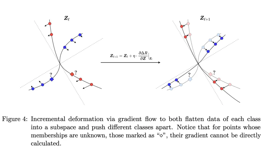
One may worry about collapse of intra-class features, but they say that neural collapse will give rise to a suboptimal overall coding rate and so is avoided.

Some Complaints

Given the novelty of the ideas of the paper, it took some time to digest and I felt some parts were under-explained, such as the reason behind why soft assignments are needed. It was also not immediately clear why we can’t keep training a single large width layer repeatedly with this setup to get good features, or experiments to show whether this was good/bad.

Concluding Thoughts

It takes a lot of determination and courage to push through novel approaches of tackling fundamental problems that people have taken for granted with traditional approaches. I think coding rate reduction is just one technique and a single step in the grander scheme of coming up with more explainable and interpretable neural network architectures that are designed from mathematical principles rather than discovered by accident, and we still have a long (but exciting) way to go in this direction.