\(\newcommand{\E}{\mathbb{E}} \newcommand{\bone}{\boldsymbol{1}} \newcommand{\bbeta}{\boldsymbol{\beta}} \newcommand{\bdelta}{\boldsymbol{\delta}} \newcommand{\bepsilon}{\boldsymbol{\epsilon}} \newcommand{\blambda}{\boldsymbol{\lambda}} \newcommand{\bomega}{\boldsymbol{\omega}} \newcommand{\bpi}{\boldsymbol{\pi}} \newcommand{\bphi}{\boldsymbol{\phi}} \newcommand{\bvphi}{\boldsymbol{\varphi}} \newcommand{\bpsi}{\boldsymbol{\psi}} \newcommand{\bsigma}{\boldsymbol{\sigma}} \newcommand{\btheta}{\boldsymbol{\theta}} \newcommand{\btau}{\boldsymbol{\tau}} \newcommand{\ba}{\boldsymbol{a}} \newcommand{\bb}{\boldsymbol{b}} \newcommand{\bc}{\boldsymbol{c}} \newcommand{\bd}{\boldsymbol{d}} \newcommand{\be}{\boldsymbol{e}} \newcommand{\boldf}{\boldsymbol{f}} \newcommand{\bg}{\boldsymbol{g}} \newcommand{\bh}{\boldsymbol{h}} \newcommand{\bi}{\boldsymbol{i}} \newcommand{\bj}{\boldsymbol{j}} \newcommand{\bk}{\boldsymbol{k}} \newcommand{\bell}{\boldsymbol{\ell}} \newcommand{\bm}{\boldsymbol{m}} \newcommand{\bn}{\boldsymbol{n}} \newcommand{\bo}{\boldsymbol{o}} \newcommand{\bp}{\boldsymbol{p}} \newcommand{\bq}{\boldsymbol{q}} \newcommand{\br}{\boldsymbol{r}} \newcommand{\bs}{\boldsymbol{s}} \newcommand{\bt}{\boldsymbol{t}} \newcommand{\bu}{\boldsymbol{u}} \newcommand{\bv}{\boldsymbol{v}} \newcommand{\bw}{\boldsymbol{w}} \newcommand{\bx}{\boldsymbol{x}} \newcommand{\by}{\boldsymbol{y}} \newcommand{\bz}{\boldsymbol{z}} \newcommand{\bA}{\boldsymbol{A}} \newcommand{\bB}{\boldsymbol{B}} \newcommand{\bC}{\boldsymbol{C}} \newcommand{\bD}{\boldsymbol{D}} \newcommand{\bE}{\boldsymbol{E}} \newcommand{\bF}{\boldsymbol{F}} \newcommand{\bG}{\boldsymbol{G}} \newcommand{\bH}{\boldsymbol{H}} \newcommand{\bI}{\boldsymbol{I}} \newcommand{\bJ}{\boldsymbol{J}} \newcommand{\bK}{\boldsymbol{K}} \newcommand{\bL}{\boldsymbol{L}} \newcommand{\bM}{\boldsymbol{M}} \newcommand{\bN}{\boldsymbol{N}} \newcommand{\bP}{\boldsymbol{P}} \newcommand{\bQ}{\boldsymbol{Q}} \newcommand{\bR}{\boldsymbol{R}} \newcommand{\bS}{\boldsymbol{S}} \newcommand{\bT}{\boldsymbol{T}} \newcommand{\bU}{\boldsymbol{U}} \newcommand{\bV}{\boldsymbol{V}} \newcommand{\bW}{\boldsymbol{W}} \newcommand{\bX}{\boldsymbol{X}} \newcommand{\bY}{\boldsymbol{Y}} \newcommand{\bZ}{\boldsymbol{Z}} \newcommand{\boldf}{\boldsymbol{f}} \newcommand{\bpi}{\boldsymbol{\pi}} \newcommand{\btheta}{\boldsymbol{\theta}} \DeclareMathOperator{\tr}{tr} \newcommand{\pdata}{p_{\text{data}}(\bx)} \newcommand{\st}{\mathbf{s}_\mathbf{\theta}} \newcommand{\xt}{\tilde{\bx}} \newcommand{\stx}{\mathbf{s}_\mathbf{\theta}(\bx)} \newcommand{\sdx}{\mathbf{s}_\text{data}(\bx)} \newcommand{\stxt}{\mathbf{s}_\mathbf{\theta}(\xt, \sigma)} \newcommand{\pv}{p_{\bv}} \newcommand{\score}{\nabla_\bx \log \pdata} \newcommand{\bov}{\bar{\beta}}\) Joint work with Owen Wang.

There has recently been a flurry of work in score-based diffusion models as part of the broader area of generative models. This is due to the recent success of such score-based methods, which has achieved results comparable to the state-of-the-art of generative adversarial networks (GANs).

Past techniques in generative modeling have either relied on the approximation of the partition function of the probability density, or the combination of an implicit network representation of the probability density and adversarial training. The former suffers from having to either constrain the model to make the partition function tractable, or otherwise relies on approximations with surrogate losses that may be inaccurate, and the latter suffers from training instability and mode collapse.

Score-based diffusion models try to address the cons of both approaches, and instead, use score-matching to learn a model of the gradient of the log of the probability density function. This allows it to avoid computing the partition function completely.

One of the first such approaches that rely on using score-matching to perform generative modeling does so by generating new samples via Langevin dynamics (Song & Ermon, 2019). A key observation is that naively applying score-matching is that the model of score function will be inaccurate in areas of low density with respect to the data distribution, which results in improper Langevin dynamics in low-density areas. The solution that was proposed is the injection of noise into the data, which provides additional training signal and increases the dimensionality of the data.

The next major step introduced in (Song et al., 2021) is to perturb the data using a diffusion process which is a form of a stochastic differential equation (SDEs). The SDE is then reversed using annealed Langevin dynamics in order to recover the generative process, where the reversal process makes use of score matching.

Other recent refinements that have been proposed include re-casting the objective as a Schrödinger bridge problem, which is an entropy-regularized optimal transport problem. The advantage of this approach is that it allows for fewer diffusion steps to be taken during the generative process.

Survey of Results

We will be primarily focusing on the paper Generative Modeling by Estimating Gradients of the Data Distribution (Song & Ermon, 2019).

In this section, we provide the necessary background, provide derivations for important results, and explain the key ideas of score matching for diffusion models as proposed in the papers.

Motivation for Score Matching

Limitations of Likelihood-Based Approaches

Score matching is motivated by the limitations of likelihood-based methods. In likelihood-based methods, we use a parameterized model \(f_\theta(\bx) \in \mathbb{R}\) and attempt it to recover the parameters \(\theta\) that best explains the observed data. For instance, in energy-based models, the probability mass function \(p_\theta(\bx)\) would be given as \begin{align} p_\theta(\bx) = \frac{\exp(-f_\theta(\bx))}{Z_\theta}, \end{align} where \(Z_\theta\) is the normalizing constant that causes the distribution to integrate to 1, i.e \begin{align} Z_\theta = \int \exp(-f_\theta(\bx)) \, d \bx. \end{align} The goal then is to maximize the log likelihood of the observed data \(\{\bx_i\}_i^N\), given by \begin{align} \max_\theta \sum_{i=1}^N \log p_\theta (\bx_i). \end{align}

It is often computationally intractable to compute the partition function \(Z_\theta\) unless there are restrictions on what the model can be, since there are usually at least an exponential number of possible configurations. Examples of models where the partition function can be efficiently computed include causal convolutions in autoregressive models, and invertible networks in normalizing flow models However, such architecture restrictions are very undesirable as they limit the expressiveness of the models.

A likelihood-based approach that tries to avoid computing the partition function is variational inference. In variational inference, we use the Evidence Lower Bound (ELBO) as a surrogate objective, where the approximation error is the smallest Kullback-Leibler divergence between the true distribution and a distribution that can be parameterized by our model.

Limitations of Adversarial-Based Approaches

Adversarial-based approaches, like generative adversarial networks (GANs), have been shown to suffer from both instability in training and mode collapse.

Training GANs can be viewed as finding a Nash equilibrium for a two-player non-cooperative game between the discriminator and the generator. Finding a Nash equilibrium is PPAD-complete which is computationally intractable, and therefore methods like gradient-based optimization techniques are used instead. However, the highly non-convex and high-dimensional optimization landscape means that small perturbations in the parameters of either player can change the cost function of the other player, which results in non-convergence.

Another problem with training GANs is that when either the generator or discriminator becomes significantly better than the other, then the learning signal for the other player becomes very weak. For generators, this is when the discriminator is always able to tell it apart. For discriminators, this is when the generator performs so well it can hardly do better than random guessing.

Finally, a common failure mode of GANs is mode collapse, where the generator only learns to produce a set of very similar outputs from a single mode instead of from all the modes. This is due to the non-convexity of the optimization landscape.

Score Matching

Score matching is a non-likelihood-based method to perform sampling on an unknown data distribution, and seeks to address many of the limitations of likelihood-based methods and adversarial methods. This is achieved by learning the score of the probability density function, formally defined below:

In practice, we try to learn the score function using a neural network \(\stx\) parameterized by \(\theta\).

The objective of score matching is to minimize the Fisher Divergence between the score function and the score network:

However, the main problem here is that we do not know \(\nabla_\bx \log \pdata\), since it depends on knowing what \(\pdata\) is.

(Hyvärinen, 2005) showed that Equation \ref{eq:score-matching-target-fisher-div} is equivalent to Equation \ref{eq:score-matching-target} below:

We can now compute this using Monte Carlo methods by sampling from \(\pdata\), since it only depends on knowing \(\stx\).

Sliced Score Matching

It is computationally difficult to compute the trace term \(\tr \left( \nabla_\bx \stx \right)\) in Equation \ref{eq:score-matching-target} when \(\bx\) is high-dimensional. This motivates another alternative cheaper approach for score matching, called sliced score matching (Song et al., 2019).

In sliced score matching, we sample random vectors from some distribution \(\pv\) (such as the multivariate standard Gaussian) in order to optimize an analog of the Fisher Divergence:

We observe that

where the \(\sdx\) term is absorbed into \(C\) as it doesn’t depend on \(\theta\). Now note

where line 16 is obtained by applying multivariate integration by parts. This finally yields the equivalent objective:

which no longer has a dependence on the unknown \(\nabla_{bx}\sdx\). This leads to the unbiased estimator:

where for each data point \(\bx_i\) we draw \(M\) projection vectors from \(\pv\).

(Song et al., 2019) showed that under some regularity conditions, sliced score matching is an asymptotically consistent estimator:

where

Sliced score matching is computationally more efficient, since it now only involves Hessian-vector products, and continues to work well in high dimensions.

Sampling with Langevin Dynamics

Once we have trained a score network, we can sample from the data distribution via Langevin dynamics. Langevin dynamics is a Markov Chain Monte Carlo method of sampling from a stationary distribution, where we can efficiently take gradients with respect to the probability of our samples \(\bx\). We satisfy this criteria since we have the trained score network.

In Langevin dynamics, we start from some initial point \(\bx_0 \sim \bpi(\bx)\) sampled from some prior distribution \(\bpi\), and then iteratively obtain updated points based on the following recurrence: \begin{align} \xt_t = \xt_{t-1} + \frac{\epsilon}{2} \nabla_\bx \log p(\xt_{t-1}) + \sqrt{\epsilon} \bz_t, \end{align} where \(\bz_t \sim \mathcal{N}(0, I)\). The addition of the Gaussian noise is required, or otherwise the process simply converges to the nearest mode instead of converging to a stationary distribution.

It can be shown that as \(\epsilon \to 0\) and \(T \to \infty\), we have that the distribution of the process \(\xt_T\) converges to \(\pdata\) (Welling & Teh, 2011).

Challenges of Langevin Dynamics

Langevin dynamics does not perform well with multi-modal distributions with poor conductance, since it will tend to stay in a single mode, which causes long mixing times. This is particularly a problem when the modes have disjoint supports, since there is very weak gradient information in the region where there is no support.

Challenges of Score Matching for Generative Modeling

The Manifold Hypothesis

The manifold hypothesis postulates that real-world data often lies in a low-dimensional manifold embedded in a high-dimensional space. This has been empirically observed in many datasets.

This poses problems for score matching. The first problem that the manifold hypothesis poses is that the score \(\score\) becomes undefined if \(\bx\) actually just lies in a low-dimensional manifold. The second problem is that the estimator in Equation \ref{eq:score-matching-target} is only consistent when the support of \(\pdata\) is that of the whole space.

In order to increase the dimension of the data to match that of the ambient space, (Hyvärinen, 2005) proposed injecting small amounts of Gaussian noise into the data, such that now the data distribution has full support. As long as the perturbation is sufficiently small (\(\mathcal{N}(0, 0.0001)\) was used in their paper), it is almost indistinguishable to humans.

Low Data Density Regions

The other problem with score matching is that it may not be able to learn the score function in areas of low data density. This is due to the lack of samples drawn from these regions, resulting in the Monte Carlo estimation to have high variance.

Noise Conditional Score Networks (NCSN)

The challenges mentioned in the previous sections are addressed by Noise Conditional Score Networks (NCSN).

In NCSN, we define a geometric sequence of \(L\) noise levels \({\left\{ \sigma_i \right\}}_{i=1}^L\), with the property that \(\frac{\sigma_1}{\sigma_2} = \frac{\sigma_{L-1}}{\sigma_L} > 1\). Each of these noise levels correspond to Gaussian noise that will be added to perturb the data distribution, i.e \(q_{\sigma_i} \sim \pdata + \mathcal{N}(0, \sigma_i)\).

We augment the score network to also take the noise level \(\sigma\) into account, which is called the NCSN \(\stxt\). The goal of NCSN is then to estimate the score conditioned on the noise level. Once we have a trained NCSN, we use a similar apporach as simulated annealing in Langevin sampling, where we begin with a large noise level in order to cross the different modes easily, before gradually annealing down the noise to achieve convergence.

The denoising score matching objective for each noise level \(\sigma_i\) is given as

and the unified objective for denoising across all levels is given as

Score-Based Generative Modeling through Stochastic Differential Equations (Song et al., 2021)

We can extend the idea of having a finite number of noise scales to having an infinite continuous number of such noise scales by modeling the process as a diffusion process, which can be formalized as a stochastic differential equation (SDE). Such an SDE is given in the following form:

Here, \(\boldf\) represents the drift coefficient, which models the deterministic part of the SDE, and determines the rate at which the process \(d\bx\) is expected to change over time on average. \(g(t)\) is called the diffusion coefficient, which represents the random part of the SDE, and determines the magnitude of the noising process over time. Finally, \(\bw\) is Brownian motion. Thus \(g(t) \, d \bw\) represents the noising process.

We want our diffusion process to be such that \(\bx(0) \sim p_0\) is the original data distribution, and \(\bx(T) \sim p_T\) is the Gaussian noise distribution that is independent of \(p_0\). Then since every SDE has a corresponding reverse SDE, we can start from the final noise distribution and run the reverse-time SDE in order to recover a sample from \(p_0\), given by the following process:

where \(\overline{w}\) is Brownian motion that flows backwards in time from \(T\) to \(0\), and \(dt\) is an infinitesimal negative timestep.

The objective function for score matching for the SDE is then given by

Score-based Generative Modeling Techniques

(Song et al., 2021) covers two score-based generative models that uses SDEs to perform generative modeling. The first is called score matching with Langevin dynamics (SMLD), which performs score estimation at different noise scales and then performs sampling using Langevin dynamics with decreasing noise scales. The second is denoising diffusion probabilistic modeling (DDPM)

(Ho et al., 2020), which uses a parameterized Markov chain that is trained with a re-weighted variant of the evidence lower bound (ELBO), which is an instance of variational inference. The Markov chain is trained to reverse the noise diffusion process, which then allows sampling from the chain using standard Markov Chain Monte Carlo techniques.

(Song et al., 2021) shows that SMLD and DDPM actually corresponds to discretizations of the Variance Exploding (VE) and Variance Preserving (VP) SDEs, which is the focus of the next two section. We believe expanding on this will be illuminating as it highlights the connections between SDEs and the discretized approaches that are used in practice.

SMLD As Discretization of Variance Exploding (VE) SDE

Recall that we use a geometric sequence of \(L\) noise levels \({\left\{ \sigma_i \right\}}_{i=1}^L\). that is added to the data distribution

We can recursively define the distribution for each noise level \(i\) by incrementally adding noise:

where \(\bz_{i-1} \sim \mathcal{N}(\mathbf{0}, \bI)\), and \(\sigma_0 = 0\) so \(\bx_0 \sim \pdata\).

If we view the noise levels as gradually changing in time, then the continuous time limit of the process is given by the following SDE: \begin{align} \bx(t + \Delta t) = \bx(t) + \sqrt{\sigma^2 (t + \Delta t ) - \sigma^2 (t)} \bz(t) \approx \bx(t) + \sqrt{\frac{d [\sigma^2 (t)]}{dt} \Delta t } \bz (t), \end{align} where the approximation holds when \(\Delta t \ll 1\). If we take \(\Delta t \to 0\), we recover the VE SDE: \begin{align} d \bx = \sqrt{\frac{d [\sigma^2 (t)]}{dt} } d \bw, \end{align} which causes the variance of \(d \bx(t)\) to go to infinity as \(t \to \infty\) due to its geometric growth, hence its name.

DDPM As Discretization of Variance Preserving (VP) SDE

Similarly, the Markov chain of the perturbation kernel of DDPM is given by \begin{align} \bx_i = \sqrt{1 - \beta_i} \bx_{i-1} + \sqrt{\beta_i} \bz_{i-1}, \qquad i = 1, \cdots, L, \end{align} where \(\left\{ \beta_i \right\}_{i=1}^L\) are the noise scales, and if we take \(L \to \infty\) with scaled noise scales \(\overline{\beta_i} = N \beta_i\), we get \begin{align} \bx_i = \sqrt{1 - \frac{\bov_i}{N} } \bx_{i-1} + \sqrt{ \frac{\bov_i}{N} } \bz_{i-1}, \qquad i = 1, \cdots, L. \end{align} Now taking limits with \(L \to \infty\), we get \begin{align} \bx(t + \Delta t) \approx \bx(t) - \frac{1}{2} \beta(t) \Delta t \bx(t) + \sqrt{\beta(t) \Delta t} \bz(t), \end{align} where the approximation comes from the second degree Taylor expansion of \(\sqrt{1 - \beta(t + \Delta t) \Delta t}\). Then taking the limit of \(\Delta t \to 0\), we obtain the VP SDE \begin{align} d \bx = - \frac{1}{2} \beta(t) \bx dt + \sqrt{\beta(t)} d \bw. \end{align} This process thus has bounded variance since \(\beta_i\) is bounded.

Experiments

We conduct the following preliminary series of experiments, based on released work by (Song & Ermon, 2019).

Investigating the manifold hypothesis

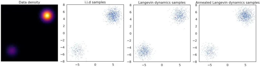
In this experiment, we have plotted the true data density of a toy distribution along with samples drawn in three ways. The i.i.d samples are drawn directly from the underlying distribution and we can see that more samples are drawn in the area of high data density. However, applying Langevin dynamics without annealing, we see that there is an almost equal number of points in the top left and bottom right corners. This is evidence that the sampling method doesn’t conform to the true distribution. Finally, by injecting and decreasing the amount of noise through the annealing process, we can recover a representative sample of the distribution.

Importance of annealing when sampling via Langevin Dynamics

To better visualize the effects of annealing when sampling via Langevin Dynamics, we generated images from a model trained on the CelebA dataset. We first tried applying Langevin Dynamics with a fixed noise and then used annealing to gradually decrease the noise.

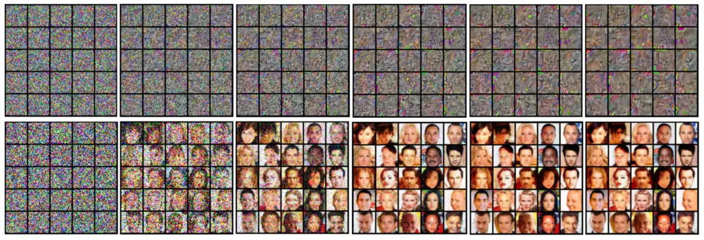
Figure 2 shows that the results with annealing are significantly clearer and more varied, matching the performance of GANs in 2019.

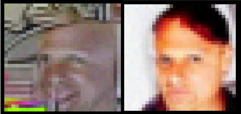
We notice that the image generated without annealing manages to produce the structure of a human face but fails to capture finer details such as the hair, and the surrounding backdrop. There is also little variation in color between different samples. This is in agreement with our theory that without annealing, Langevin dynamics cannot properly explore regions of lower data density.

Effect of noise parameters for annealed Langevin Dynamics

We also investigated the effect of changing the lowest noise standard deviation \(\sigma\) while keeping the number of different noises injected fixed at \(10\). The 10 noise values are determined by an interpolation in log scale.

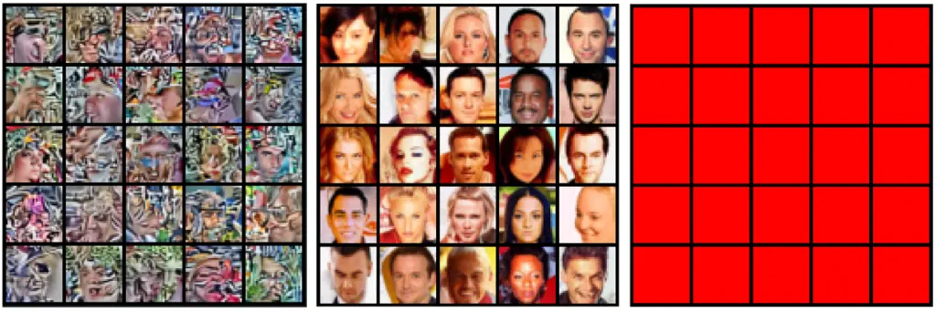
Our experiment shows that the effect of starting, ending, and the interval between noise values has a significant effect on the convergence of annealed Langevin sampling.

Discussion and Future Work

Having completed a survey of score-based diffusion models, and having run some experiments on them, we now turn our attention to discussing the pros and cons of this approach.

As mentioned previously in this paper, the main draw of score-based diffusion models is that it has shown to be capable of generating impressive high-quality samples that is on-par with the state-of-the-art with GANs. We hence focus on its limitations and how they might be overcome, drawing from work in (Cao et al., 2022).

Computation Cost

A common refrain of score-based diffusion model is the high computational complexity in both training and sampling. This is because it requires thousands of small diffusion steps in order to ensure that the forward and reverse SDEs hold in their approximations (Zheng et al., 2022). If the diffusion steps are too large, then the Gaussian noise assumption may not hold, resulting in poor score estimates. This makes it significantly more expensive than other generative methods like GANs and VAEs. To this end, there are some directions being explored to improve its computation cost.

The first technique seeks to reduce the number of sampling steps required by a method known as knowledge distillation (Lopes et al., 2017). In knowledge distillation, knowledge is transferred from a larger and more complex model (called the teacher), to one that is smaller and simpler (called the student). This technique has found success in other domains such as image classification, and has also been shown to result in improvements in diffusion models (Salimans & Ho, 2022). It would be interesting to see how far we can take this optimization.

Another technique known as truncated diffusion probabilistic modeling (TDPM) (Zheng et al., 2022). In this approach, instead of considering the diffusion process until it becomes pure noise, the process is stopped once it reaches a hidden noisy-data distribution that can be learnt by an auto-encoder by adversarial training. Then in order to produce samples, a sample is first drawn from the learnt noisy-data distribution, before being passed through the reverse-SDE diffusion steps.

It also suffers from poor explainability and interpretability, but this is a common problem across other generative models.

(Song et al., 2021) also notes that it is currently difficult to tune the myriad of hyperparameters introduced by the choice of noise levels and specific samplers chosen, and new methods to automatically select and tune these hyperparameters would make score-based diffusion models more easily deployable in practice.

Modality Diversity

Diffusion models have mostly only seen applications for generating image data, and its potential for generating other data modalities has not been as thoroughly investigated. (Austin et al., 2021) introduces Discrete Denoising Diffusion Probabilistic Models (D3PMs), which develops a diffusion process for corrupting text data into noise. It would be interesting to see how well diffusion models can be stretched to perform compared to state-of-the-art transformer models in text generation.

Dimensionality Reduction

Dimensionality reduction is another technique that can be used to speed up training and sampling speeds of diffusion models. Diffusion models are typically trained directly in data space. (Vahdat et al., 2021) instead proposes for them to be trained in latent space, which results in dimensionality reduction in the representation learnt, and also potentially increases the expressiveness of the framework. In a similar vein, (Zhang et al., 2022) argues that due to redundancy in spatial data, it is not necessary to learn in data space, and instead proposes a dimensionality-varying diffusion process (DVDP), where the dimensionality of the signal is dynamically adjusted during the both the diffusion and denoising process.

Conclusion

We showed that score matching presents a promising new direction for generative models, which avoids many of the limitations of other approaches such as training instability and mode collapse in GANs, and poor approximation guarantees in variational inference. While score matching has several flaws, such as suffering from the manifold hypothesis and requiring an expensive Langevin dynamics process in order to draw samples, successive work has done well in addressing these limitations to make score matching on diffusion models a viable contender to displace GANs as the state-of-the-art for generative modeling.

Our experiments in this blog post help to provide empirical context to the theoretical results we have derived. Most notably, we have shown how annealing is an essential part of sampling via Langevin dynamics.

Finally, we discuss some future directions that can help to improve the viability of using score-based diffusion models, which includes improving its computational cost in both training and sampling and increasing the diversity of applicable modalities.

Citation

@article{zeng2023diffusion,
  title   = {Score-Based Diffusion Models},
  author  = {Fan Pu Zeng and Owen Wang},
  journal = {fanpu.io},
  year    = {2023},
  month   = {Jun},
  url     = {https://fanpu.io/blog/2023/score-based-diffusion-models/}
}

References

• Austin, J., Johnson, D. D., Ho, J., Tarlow, D., and van den Berg, R. Structured denoising diffusion models in discrete state-spaces. CoRR, abs/2107.03006, 2021.
• Cao, H., Tan, C., Gao, Z., Chen, G., Heng, P.-A., and Li, S. Z. A survey on generative diffusion model, 2022.
• Ho, J., Jain, A., and Abbeel, P. Denoising diffusion probabilistic models. CoRR, abs/2006.11239, 2020. URL https://arxiv.org/abs/2006.11239.
• Hyva ̈rinen, A. Estimation of non-normalized statistical models by score matching. Journal of Machine Learning Research, 6(24):695–709, 2005.
• Lopes, R. G., Fenu, S., and Starner, T. Data-free knowledge distillation for deep neural networks. CoRR, abs/1710.07535, 2017.
• Salimans, T. and Ho, J. Progressive distillation for fast sampling of diffusion models. CoRR, abs/2202.00512, 2022.
• Song, Y. and Ermon, S. Generative modeling by estimating gradients of the data distribution. CoRR, abs/1907.05600, 2019.
• Song, Y., Garg, S., Shi, J., and Ermon, S. Sliced score matching: A scalable approach to density and score estimation. CoRR, abs/1905.07088, 2019. URL http://arxiv.org/abs/1905.07088.
• Song, Y., Sohl-Dickstein, J., Kingma, D. P., Kumar, A., Ermon, S., and Poole, B. Score-based generative modeling through stochastic differential equations. ICLR, abs/1907.05600, 2021.
• Vahdat, A., Kreis, K., and Kautz, J. Score-based generative modeling in latent space, 2021.
• Welling, M. and Teh, Y. W. Bayesian learning via stochastic gradient langevin dynamics. In Proceedings of the 28th International Conference on International Conference on Machine Learning, ICML’11, pp. 681–688, Madison, WI, USA, 2011. Omnipress. ISBN 9781450306195.
• Zhang, H., Feng, R., Yang, Z., Huang, L., Liu, Y., Zhang, Y., Shen, Y., Zhao, D., Zhou, J., and Cheng, F. Dimensionality-varying diffusion process, 2022.
• Zheng, H., He, P., Chen, W., and Zhou, M. Truncated diffusion probabilistic models and diffusion-based adversarial auto-encoders, 2022.