\[\newcommand{\rcal}{\mathcal{R}} \newcommand{\lcal}{\mathcal{L}} \newcommand{\mcal}{\mathcal{M}} \newcommand{\mocal}{\overline{\mathcal{M}}} \newcommand{\mocalp}{\overline{\mathcal{M}}^\perp} \newcommand{\mcalp}{\mathcal{M}^\perp} \newcommand{\sse}{\subseteq} \newcommand{\kl}{\kappa_{\lcal}} \newcommand{\tl}{\tau_{\lcal}} \newcommand{\ts}{\theta^*} \newcommand{\hd}{\widehat{\Delta}} \newcommand{\thatn}{\hat{\theta}_n} \newcommand{\that}{\hat{\theta}} \newcommand{\thatlambda}{\widehat{\theta}_{\lambda_n}} \newcommand{\thatl}{\thatlambda} \newcommand{\rs}{\rcal^*} \newcommand{\ctriplet}{ \C(\mcal, \mocalp; \ts) } \newcommand{\fcal}{\mathcal{F}} \newcommand{\kbb}{\mathbb{K}} \newcommand{\dotprod}[2]{\langle #1, #2 \rangle} \DeclareMathOperator*{\argmin}{arg\,min}\]

Introduction

In high-dimensional statistical inference, it is common for the number of parameters $p$ to be comparable to or greater than the sample size $n$. However, for an estimator $\thatn$ to be consistent in such a regime, meaning that it converges to the true parameter $\theta$, it is necessary to make additional low-dimensional assumptions on the model. Examples of such constraints that have been well-studied include linear regression with sparsity constraints, estimation of structured covariance or inverse covariance matrices, graphical model selection, sparse principal component analysis (PCA), low-rank matrix estimation, matrix decomposition problems and estimation of sparse additive nonparametric models (Negahban et al., 2009).

In recent years, there has been a flurry of work on each of these individual specific cases. However, the authors of the paper in discussion poses the question of whether there is a way of unifying these analysis to understand all of such estimators in a common framework, and answers it in the affirmative. They showed that it is possible to bound the squared difference between any regularized $M$-estimator and its true parameter by (1) the decomposability of the regularization function, and (2) restricted strong convexity of the loss function. We will call this the “main theorem” in the remainder of the blog post, and this is referred to as “Theorem 1” in (Negahban et al., 2009).

In the remainder of the paper, we will develop the tools necessary to deeply understand and prove the result. Notation used will be consistent with the original paper for expositional clarity.

Background

In this section, we develop some of the necessary background and notation to build up to the proof.

Regularized $M$-estimators

$M$-estimators ($M$ for “maximum likelihood-type”) are solutions that minimize the sum of loss functions $\rho$: \begin{align} \that \in \argmin_\theta \sum_{i=1}^n \rho(x_i, \theta). \end{align}

If we add a regularization term $\rcal$ to penalize complexity of the model, scaled by weights $\lambda$, the method is known as a regularized $M$-estimator: \begin{align} \that \in \argmin_\theta \sum_{i=1}^n \rho(x_i, \theta) + \lambda \rcal(\theta). \end{align}

Example (Lasso Program)

The Lasso program is an example of a regularized $ M $-estimator, where a $ \ell_1 $ regularization penalty is applied: $$ \that \in \argmin_{\theta \in \mathbb{R}^d} \left\{ \frac{1}{2n} \| y - \bX \theta \|_2^2 + \lambda_n \| \theta \|_1 \right\}. $$

Dual Norms

Definition (Dual Norms)

Let $\rcal$ be a norm induced by an inner product $\dotprod{\cdot}{\cdot}$. Then the dual norm of $\rcal$ is defined as $$ \rs(v) \coloneqq \sup_{u \in \mathbb{R}^p \setminus \left\{ 0 \right\}} \frac{ \dotprod{u}{v} }{\rcal (u)} = \sup_{\rcal(u) \leq 1} \dotprod{u}{v}. $$

Example ($\ell_1$ and $\ell_\infty$ norms are dual norms)

We will show that the dual of the $ \ell_1 $ norm is the $ \ell_\infty $ norm. Well, to see that $ \rs(v) \leq \| v \|_\infty $, observe that \begin{align*} \rs(v) & = \sup_{\| u \|_1 \leq 1} \dotprod{u}{v} \\ & = \sup_{\| u \|_1 \leq 1} \sum_{k=1}^p | u_k | | v_k | \\ & \leq \sup_{\| u \|_1 \leq 1} \left( \sum_{k=1}^p | u_k | \right) \| v \|_\infty \\ & = | v |_\infty \tag{since $ \| u \|_1 \leq 1 $ }. \end{align*} For the opposite direction, \begin{align*} \sup_{\| u \|_1 \leq 1} \dotprod{u}{v} & = \sup_{\| u \|_1 \leq 1} \sum_{k=1}^p |u_k| |v_k| \\ & \geq 1 \cdot |v_j| \tag{ set $ j = \argmax_j |v_j|, u = \be_j $ } \\ & = \| v \|_\infty, \end{align*} hence we have equality.

Subspace Compatibility Constant

The subspace compatibility constant measures how much the regularizer $\rcal$ can change with respect to the error norm $\| \cdot \|$ restricted to the subspace $\mcal$. This concept will show up later in showing that the restricted strong convexity condition will hold with certain parameters.

The subspace compatibility constant is defined as follows:

Definition (Subspace Compatibility Constant)

For any subspace $ \mcal $ of $ \mathbb{R}^p $, the subspace compatibility constant with respect to the pair $ (\rcal, \| \cdot \|) $ is given by $$ \varPsi (\mcal) \coloneqq \sup_{u \in \mcal \setminus \left\{ 0 \right\}} \frac{\rcal(u)}{\| u \|}. $$

It can be thought of as the Lipschitz constant of the regularizer with respect to the error norm restricted to values in $\mcal$, by considering the point where it can vary the most.

Projections

Define the projection operator \begin{align} \Pi_{\mcal}(u) \coloneqq \argmin_{v \in \mcal} | u - v | \end{align} to be the projection of $u$ onto the subspace $\mcal$. For notational brevity, we will use the shorthand $u_{\mcal} = \Pi_{\mcal}(u)$.

One property of the projection operator is that it is non-expansive, meaning that \begin{align} | \Pi(u) - \Pi(v) | \leq | u - v | \label{eq:non-expansive} \end{align} for some error norm $\| \cdot \|$. In other words, it has Lipschitz constant 1.

Problem Formulation

In our setup, we define the following quantities:

$Z_1^n \coloneqq \left\{ Z_1, \cdots, Z_n \right\}$ $n$ i.i.d observations drawn from distribution $\mathbb{P}$ with some parameter $\theta^*$,
$\mathcal{L}: \mathbb{R}^p \times \mathcal{Z}^n \to \mathbb{R}$ a convex and differentiable loss function, such that $\mathcal{L}(\theta; Z_1^n)$ returns the loss of $\theta$ on observations $Z_1^n$,
$\lambda_n > 0$: a user-defined regularization penalty,
$\mathcal{R} : \mathbb{R}^p \to \mathbb{R}_+$ a norm-based regularizer.

The purpose of the regularized $M$-estimator is then to solve for the convex optimization problem

\[\begin{align} \label{eq:opt} \widehat{\theta}_{\lambda_n} \in \argmin_{\theta \in \mathbb{R}^p} \left\{ \mathcal{L}(\theta; Z_1^n) + \lambda_n \mathcal{R} (\theta) \right\}, \end{align}\]

and we are interested in deriving bounds on $\begin{align} \| \thatlambda - \theta^* \| \end{align}$ for some error norm $\| \cdot \|$ induced by an inner product $\langle \cdot, \cdot \rangle$ in $\mathbb{R}^p$.

Decomposability of the Regularizer $\mathcal{R}$

The first key property in the result is decomposability of our norm-based regularizer $\rcal$. Working in the ambient $\mathbb{R}^p$, define $\mcal \sse \mathbb{R}^p$ to be the model subspace that captures the constraints of the model that we are working with (i.e $k$-sparse vectors), and denote $\mocal$ to be its closure, i.e the union of $\mcal$ and all of its limit points. In addition, denote $\mocalp$ to be the orthogonal complement of $\mocal$, namely

\[\begin{align} \mocalp \coloneqq \left\{ v \in \mathbb{R}^p \mid \langle u, v \rangle = 0 \text{ for all $ u \in \mocal $ } \right\}. \end{align}\]

We call this the perturbation subspace, as they represent perturbations away from the model subspace $\mocal$. The reason why we need to consider $\mocal$ instead of $\mcal$ is because there are some special cases of low-rank matrices and nuclear norms where it could be possible that $\mcal$ is strictly contained in $\mocal$.

Now we can introduce the property of decomposability:

Definition (Regularizer Decomposability)

Given a pair of subspaces $ \mcal \sse \mocal $, a norm-based regularizer $ \rcal $ is decomposable with respect to $ (\mocal, \mocalp) $ if $$ \rcal(\theta + \gamma) = \rcal(\theta) + \rcal(\gamma) $$ for all $ \theta \in \mcal $ and $ \gamma \in \mocalp $.

Since $\rcal$ is a norm-based regularizer, by the triangle inequality property of norms we know that always \begin{align} \rcal(\theta + \gamma) \leq \rcal(\theta) + \rcal(\gamma), \end{align} and hence this is a stronger condition which requires tightness in the inequality when we are specifically considering elements in the closure of the model subspace and its orthogonal complement.

Decomposability of the regularizer is important as it allows us to penalize deviations $\gamma$ away from the model subspace in $\mcal$ to the maximum extent possible. We are usually interested to find model subspaces that are small, with a large orthogonal complement. We will see in the main theorem that when this is the case, we will obtain better rates for estimating $\theta^*$.

There are many natural contexts that admit regularizers which are decomposable with respect to subspaces, and the following example highlights one such case.

Example ($ s $-sparse Vectors)

Consider estimating the parameters $ \that $ with $ \ell_1 $-regularization in $ \mathbb{R}^p $ where we assume that the model is $ s $-sparse. Then for any set $ S \sse [p] $ where $ |S| = s $, we can define our model subspace $ \mcal $ as \[ \begin{align*} \mcal(S) \coloneqq \left\{ \theta \in \mathbb{R}^p \mid \theta_j = 0 \quad \forall j \not\in S \right\}, \end{align*} \] i.e all the vectors in $ \mathbb{R}^p $ that only has support in $ S $. In this case, $ \mcal = \mocal $, and our orthogonal complement $ \mocalp $ is just \[ \begin{align*} \mocalp(S) \coloneqq \left\{ \gamma \in \mathbb{R}^p \mid \gamma_j = 0 \quad \forall j \in S \right\}. \end{align*} \] Then this setup is decomposable: \[ \begin{align*} \| \theta + \gamma \|_1 = \| \theta_S + \gamma_{S^c} \|_1 = \| \theta_S \|_1 + \| \gamma_{S^c} \| = \| \theta \|_1 + \| \gamma \|_1 \end{align*} \] by the Pythagorean theorem.

Role of Decomposability

*Figure 1.* A visualization of $ \ctriplet $. The shaded area represents the set $ \ctriplet $, i.e all values of $ \theta $ that satisfies the inequality of the set in Lemma 1.

Decomposability is important because it allows us to bound the error of the estimator. This is given in the following result, which is known as Lemma 1 in (Negahban et al., 2009):

Lemma (Lemma 1 in (Negahban et al., 2009) )

Suppose that $ \lcal $ is a convex and differentiable function, and consider any optimal solution $ \that $ to the optimization problem with a strictly positive regularization parameter satisfying $$ \begin{align*} \lambda_n \geq 2 \rcal^* (\nabla \lcal (\ts; Z_1^n)). \end{align*} $$ Then for any pair $ (\mcal, \mocalp) $ over which $ \rcal $ is decomposable, the error $ \hd = \thatlambda - \ts $ belongs to the set $$ \begin{align*} \label{eq:c} \C(\mcal, \mocalp; \ts) \coloneqq \left\{ \Delta \in \mathbb{R}^p \mid \rcal(\Delta_{\mocalp}) \leq 3 \rcal (\Delta_{\mocal}) + 4 \rcal (\ts_{\mcalp}) \right\}. \end{align*} $$

Recall from the Projections Section that $\Delta_{\mocalp}$ represents the projection of $\Delta$ onto $\mocalp$, and similarly for the other quantities. Due to space constraints, we are unable to prove Lemma Lemma 1 in this survey, but it is very important in the formulation of restricted strong convexity, and in proving Theorem 1.

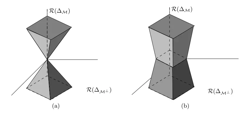
Figure 1 provides a visualization of $\ctriplet$ in $\mathbb{R}^3$ in the sparse vectors setting. In this case, $S = \left\{ 3 \right\}$ with $|S|=1$, and so the projection of $\Delta$ onto the model subspace only has non-zero values on the third coordinate, and its orthogonal complement is where the third coordinate is zero. Formally,

\[\begin{align} \mcal(S) = \mocal(S) & = \left\{ \Delta \in \mathbb{R}^3 \mid \Delta_1 = \Delta_2 = 0 \right\}, \\ \mocalp(S) & = \left\{ \Delta \in \mathbb{R}^3 \mid \Delta_3 = 0 \right\}. \end{align}\]

The vertical axis of Figure 1 denotes the third coordinate, and the horizontal plane denotes the first two coordinates. The shaded area represents the set $\ctriplet$, i.e all values of $\theta$ that satisfies the inequality of the set in Lemma 1.

Figure 1(a) shows the special case when $\ts \in \mcal$. In this scenario, $\rcal (\ts_{\mcalp}) = 0$, and so

\[\begin{align*} \C(\mcal, \mocalp; \ts) = \left\{ \Delta \in \mathbb{R}^p \mid \rcal(\Delta_{\mocalp}) \leq 3 \rcal (\Delta_{\mocal}) \right\}, \end{align*}\]

which is a cone.

However, in the general setting where $\ts \not\in \mcal$, then $\rcal (\ts_{\mcalp}) > 0$, and the set $\ctriplet$ will become a star-shaped set like what is shown in Figure 1(b).

Restricted Strong Convexity (RSC) of the Loss Function

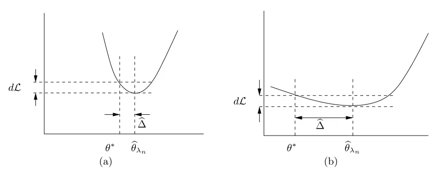
*Figure 2.* An illustration of the role of curvature in guaranteeing that $ \hd = \thatlambda - \ts $ is small when $ \lcal(\thatlambda) - \lcal(\ts) $ is small.

In a classical setting, as the number of samples $n$ increases, the difference in loss $d \lcal = |\lcal(\thatlambda) - \lcal(\ts)|$ will converge to zero. However, the convergence in loss by itself is insufficient to also ensure the convergence in parameters, $\hd = \thatlambda - \ts$. Instead, it also depends on the curvature of the loss function $\lcal$.

Figure 2 illustrates the importance of curvature. In Figure 2(a), $\lcal$ has high curvature, and so having a small $d\lcal$ also implies a small $\hd$. On the other hand, in Figure 2(b), $\lcal$ has an almost flat landscape near $\thatlambda$, and hence even when $d \lcal$ is small, $\hd$ could still be large.

Consider performing a Taylor expansion of $\lcal$ around $\ts$:

\[\begin{align} \lcal(\ts + \Delta) & = \lcal(\ts) + \dotprod{\nabla \lcal(\ts)}{\Delta} + \underbrace{\frac{1}{2} \Delta^T \nabla^2 \lcal(\ts) \Delta + \dots}_{\delta \lcal(\Delta, \ts)}. \end{align}\]

Then we can rearrange and write the error of the first-order Taylor series expansion at $\ts$ as

\[\begin{align*} \delta \lcal(\Delta, \ts) = \lcal(\ts + \Delta) - \lcal(\ts) - \dotprod{\nabla \lcal(\ts)}{\Delta}. \end{align*}\]

The first-order Taylor approximation is a linear approximation, and hence the error $\delta \lcal(\Delta, \ts)$, which is dominated by the quadratic term, can capture the curvature about $\ts$.

As such, one way to show that $\lcal$ has good curvature about $\ts$ is to show that $\delta \lcal(\Delta, \ts) \geq \kappa \|\Delta \|^2$ holds for all $\Delta$ in a neighborhood of $\ts$. This is because we are enforcing a lower bound on its quadratic growth.

This leads us to the definition of restricted strong convexity:

Definition (Restricted Strong Convexity)

The loss function satisfies a restricted strong convexity (RSC) condition with curvature $ \kl > 0 $ and tolerance function $ \tl $ if \begin{align*} \delta \lcal(\Delta, \ts) \geq \kl \| \Delta \|^2 - \tl^2(\ts) \end{align*} for all $ \Delta \in \ctriplet $.

We only need to consider error terms $\Delta \in \ctriplet$, since Lemma \ref{lemma:1} guarantees us that the error term will only lie in that set.

In many statistical models, restricted strong convexity holds with $\tl = 0$, however, it is required in more general settings, such as generalized linear models.

Proof of Theorem 1

We can now state and prove the main result of the paper. This will hold under the decomposability of the regularizer (G1), and the restricted strong convexity of the loss function (G2).

(G1) The regularizer $\rcal$ is a norm and is decomposable with respect to the subspace pair $(\mcal, \mocalp)$, where $\mcal \sse \mocalp$.
(G2) The loss function $\lcal$ is convex and differentiable, and satisfies restricted strong convexity with curvature $\kl$ and tolerance $\tl$.

Theorem 1 in (Negahban et al., 2009) (Bounds for General Models)

Under conditions (G1) and (G2), consider the convex optimization problem (\ref{eq:opt}) based on a strictly positive positive regularization constant $ \lambda_n \geq 2 \rs (\nabla \lcal (\ts)) $. Then any optimal solution $ \thatlambda $ to the convex program (\ref{eq:opt}) satisfies the bound \begin{align*} \| \thatlambda - \ts \|^2 \leq 9 \frac{\lambda_n^2}{\kl^2} \Psi^2(\mocal) + \frac{\lambda_n}{\kl} \left( 2 \tl^2 (\ts) + 4 \rcal (\ts_{\mcal^{\perp}}) \right). \end{align*}

We will rely on the following lemmas that will be stated without proof due to space constraints:

Lemma 3 in (Negahban et al., 2009) (Deviation Inequalities)

For any decomposable regularizer and $ p $-dimensional vectors $ \ts $ and $ \Delta $, we have \begin{align*} \rcal(\ts + \Delta) - \rcal(\ts) \geq \rcal(\Delta_{\mocalp}) - \rcal(\Delta_{\mocal}) - 2 \rcal(\ts_{\mcal^{\perp}}). \end{align*} Moreover, as long as $ \lambda_n \geq 2 \rs (\nabla \lcal(\ts)) $ and $ \lcal $ is convex, we have \begin{align*} \lcal(\ts + \Delta) - \lcal(\ts) \geq - \frac{\lambda_n}{2} [\rcal(\Delta_{\mocal}) + \rcal(\Delta_{\mocalp})]. \end{align*}

Lemma 4 in (Negahban et al., 2009)

If $ \fcal(\Delta) > 0 $ for all vectors $ \Delta \in \mathbb{K}(\delta) $, then $ \| \hd \| \leq \delta $.

Note that this was similar to our previous analysis on restricted strong convexity where we only really need to consider error terms restricted to $\ctriplet$ due to Lemma 1. Therefore, it suffices to show $\fcal(\Delta) > 0$ to obtain a bound on $\| \hd \| = \| \thatlambda - \ts\|$, which completes the proof of Theorem 1.

Define $\fcal : \mathbb{R}^p \to \mathbb{R}$ by

\[\begin{align} \fcal(\Delta) \coloneqq \lcal(\ts + \Delta) - \lcal(\ts) + \lambda_n \left\{ \rcal(\ts + \Delta) - \rcal(\ts) \right\}, \end{align}\]

and define the set

\[\begin{align} \mathbb{K}(\delta) \coloneqq \ctriplet \cap \left\{ \| \Delta \| = \delta \right\}. \end{align}\]

Take any $\Delta \in \kbb$. Then

\[\begin{align} \fcal(\Delta) = & \lcal(\ts + \Delta) - \lcal(\ts) + \lambda_n \left\{ \rcal(\ts + \Delta) - \rcal(\ts) \right\} \tag{by definition} \\ \geq & \langle \nabla \lcal (\ts), \Delta \rangle + \kl \| \Delta \|^2 - \tl^2(\ts) + \lambda_n \left\{ \rcal(\ts + \Delta) - \rcal(\ts) \right\} \\ & \qquad \text{(by restricted strong convexity: $\delta \lcal(\Delta, \ts) \geq \kl \| \Delta \|^2 - \tl^2(\ts)$,} \\ & \qquad \text{ and $ \delta \lcal(\Delta, \ts) = \lcal(\ts + \Delta) - \lcal(\ts) - \dotprod{\nabla \lcal(\ts)}{\Delta} $ ) } \\ \geq & \langle \nabla \lcal (\ts), \Delta \rangle + \kl \| \Delta \|^2 - \tl^2(\ts) + \lambda_n \left\{ \rcal(\Delta_{\mocalp}) - \rcal(\Delta_{\mocal}) - 2 \rcal(\ts_{\mcal^{\perp}}) \right\} \\ & \qquad \text{(by Lemma 3)}. \label{thm-deriv:1} \end{align}\]

We lower bound the first term as $\langle \nabla \lcal (\ts), \Delta \rangle \geq - \frac{\lambda_n}{2} \rcal(\Delta)$:

\[\begin{align} | \langle \nabla \lcal (\ts), \Delta \rangle | \leq & \rs(\nabla \lcal(\ts)) \rcal(\Delta) & \text{(Cauchy-Schwarz using dual norms $ \rcal $ and $ \rs $)} \\ \leq & \frac{\lambda_n}{2} \rcal(\Delta) & \text{Theorem 1 assumption: $ \lambda_n \geq 2 \rs (\nabla \lcal(\ts)) $)}, \end{align}\]

and hence,

\[\begin{align} \langle \nabla \lcal (\ts), \Delta \rangle \geq & - \frac{\lambda_n}{2} \rcal(\Delta). \end{align}\]

So applying to (\ref{thm-deriv:1}),

\[\begin{align} \fcal(\Delta) \geq & \kl \| \Delta \|^2 - \tl^2(\ts) + \lambda_n \left\{ \rcal(\Delta_{\mocalp}) - \rcal(\Delta_{\mocal}) - 2 \rcal(\ts_{\mcal^{\perp}}) \right\} - \frac{\lambda_n}{2} \rcal(\Delta) \\ \geq & \kl \| \Delta \|^2 - \tl^2(\ts) + \lambda_n \left\{ \rcal(\Delta_{\mocalp}) - \rcal(\Delta_{\mocal}) - 2 \rcal(\ts_{\mcal^{\perp}}) \right\} - \frac{\lambda_n}{2} (\rcal(\Delta_{\mocalp}) + \rcal(\Delta_{\mocal})) \\ & \qquad \text{(Triangle inequality: $ \rcal(\Delta) \leq \rcal(\Delta_{\mocalp}) + \rcal(\Delta_{\mocal}) $)} \\ = & \kl \| \Delta \|^2 - \tl^2(\ts) + \lambda_n \left\{ \frac{1}{2}\rcal(\Delta_{\mocalp}) - \frac{3}{2}\rcal(\Delta_{\mocal}) - 2 \rcal(\ts_{\mcal^{\perp}}) \right\} \\ & \qquad \text{(Moving terms in)} \\ \geq & \kl \| \Delta \|^2 - \tl^2(\ts) + \lambda_n \left\{ - \frac{3}{2}\rcal(\Delta_{\mocal}) - 2 \rcal(\ts_{\mcal^{\perp}}) \right\} \\ & \qquad \text{(Norms always non-negative)} \\ = & \kl \| \Delta \|^2 - \tl^2(\ts) - \frac{\lambda_n }{2} \left\{ 3 \rcal(\Delta_{\mocal}) + 4 \rcal(\ts_{\mcal^{\perp}}) \right\} \label{eq:r-delta-lb} . \end{align}\]

To bound the term $\rcal(\Delta_{\mocal})$, recall the definition of subspace compatibility:

\[\begin{align} \varPsi (\mcal) \coloneqq \sup_{u \in \mcal \setminus \left\{ 0 \right\}} \frac{\rcal(u)}{\| u \|}, \label{eq:r-delta-ub} \end{align}\]

and hence

\[\begin{align} \rcal(\Delta_{\mocal}) \leq \varPsi(\mocal) \| \Delta_{\mocal} \|. \end{align}\]

To upper bound $\| \Delta_{\mocal} \|$, we have

\[\begin{align} \| \Delta_{\mocal} \| & = \| \Pi_{\mocal} (\Delta) - \Pi_{\mocal}(0) \| & \text{(Since $0 \in \mocal $, $ \Pi_{\mocal}(0) = 0 $) } \\ & \leq \| \Delta - 0 \| & \text{(Projection operator is non-expansive, see Equation \ref{eq:non-expansive})} \\ & = \| \Delta \|, \end{align}\]

which substituting into Equation (\ref{eq:r-delta-ub}) gives

\[\begin{align} \rcal(\Delta_{\mocal}) \leq \varPsi(\mocal) \| \Delta \|. \end{align}\]

Now we can use this result to lower bound Equation \ref{eq:r-delta-lb}:

\[\begin{align} \fcal (\Delta) \geq & \kl \| \Delta \|^2 - \tl^2(\ts) - \frac{\lambda_n }{2} \left\{ 3 \varPsi(\mocal) \| \Delta \| + 4 \rcal(\ts_{\mcal^{\perp}}) \right\}. \label{eq:strict-psd} \end{align}\]

The RHS of the inequality in Equation \ref{eq:strict-psd} has a strictly positive definite quadratic form in $\| \Delta \|$, and hence by taking $\| \Delta \|$ large, it will be strictly positive. To find such a sufficiently large $\| \Delta \|$, write

\[\begin{align} a & = \kl, \\ b & = \frac{3\lambda_n}{2} \varPsi (\mocal), \\ c & = \tau_{\lcal}^2 (\ts) + 2 \lambda_n \rcal(\ts_{\mcalp}), \\ \end{align}\]

such that we have

\[\begin{align} \fcal (\Delta) & \geq a \| \Delta \|^2 - b \| \Delta \| - c. \end{align}\]

Then the square of the rightmost intercept is given by the squared quadratic formula

\[\begin{align} \| \Delta \|^2 & = \left( \frac{-(-b) + \sqrt{b^2 - 4a(-c)}}{2a} \right)^2 \\ & = \left( \frac{b + \sqrt{b^2 + 4ac}}{2a} \right)^2 \\ & \leq \left( \frac{\sqrt{b^2 + 4ac}}{a} \right)^2 & \text{($b \leq \sqrt{b^2 + 4ac}$)} \label{eq:coarse-bound} \\ & = \frac{b^2 + 4ac}{a^2} \\ & = \frac{9 \lambda_n^2 \varPsi^2 (\mocal)}{4 \kl^2} + \frac{ 4 \tau_{\lcal}^2 (\ts) + 8 \lambda_n \rcal(\ts_{\mcalp}) }{\kl}. & \text{(Substituting in $a, b, c$)} \\ \end{align}\]

In (Negahban et al., 2009), they were able to show an upper bound of

\[\begin{align} \| \Delta \|^2 & \leq \frac{9 \lambda_n^2 \varPsi^2 (\mocal)}{\kl^2} + \frac{\lambda_n}{\kl} \left\{ 2\tau_{\lcal}^2 (\ts) + 4 \rcal(\ts_{\mcalp}) \right\}, \label{eq:ub} \end{align}\]

but I did not manage to figure out how they managed to produce a $\lambda_n$ term beside the $\tl^2(\ts)$ term. All other differences are just constant factors. It may be due to an overly coarse bound on my end applied in Equation \ref{eq:coarse-bound}, but it is unclear to me how the $\lambda_n$ term can be applied on only the $\tl^2(\ts)$ term without affecting the $\rcal(\ts_{\mcalp})$ term.

With Equation \ref{eq:ub}, we can hence apply Lemma 4 in (Negahban et al., 2009) to obtain the desired result that

\[\begin{align} \| \thatlambda - \ts \|^2 \leq 9 \frac{\lambda_n^2}{\kl^2} \Psi^2(\mocal) + \frac{\lambda_n}{\kl} \left( 2 \tl^2 (\ts) + 4 \rcal (\ts_{\mcal^{\perp}}) \right). \end{align}\]

This concludes the proof.

Conclusion

In the proof of Theorem 1, we saw how the bound is derived from the two key ingredients of the decomposability of the regularizer, and restricted strong convexity of the loss function. The decomposability of the regularizer allowed us to ensure that the error vector $\hd$ will stay in the set $\ctriplet$. This condition is then required in Lemma 4 of (Negahban et al., 2009), which allows us to bound $\| \hd \|$ given that $\fcal(\Delta) > 0$. In one of the steps where we were lower bounding $\fcal(\Delta)$ in the proof, we made use of the properties of restricted strong convexity.

Theorem 1 provides a family of bounds for each decomposable regularizer under the choice of $(\mcal, \mocalp)$. The authors of (Negahban et al., 2009) were able to use Theorem 1 to rederive both existing known results, and also derive new results on low-rank matrix estimation using the nuclear norm, minimax-optimal rates for noisy matrix completion, and noisy matrix decomposition. The reader is encouraged to refer to (Negahban et al., 2009) for more details on the large number of corrollaries of Theorem 1.

Acknowledgments

I would like to thank my dear friend Josh Abrams for helping to review and provide valuable suggestions for this post!

Citations

Negahban, S., Yu, B., Wainwright, M. J., and Ravikumar, P. A unified framework for high-dimensional analysis of m-estimators with decomposable regularizers. In Bengio, Y., Schuurmans, D., Lafferty, J., Williams, C., and Culotta, A. (eds.), Advances in Neural Information Processing Systems, volume 22. Curran Associates, Inc., 2009. URL https://proceedings.neurips.cc/paper_files/paper/2009/file/dc58e3a306451c9d670adcd37004f48f-Paper.pdf.

A Unified Framework for High-Dimensional Analysis of M-Estimators with Decomposable Regularizers: A Guided Walkthrough