The Art of LaTeX: Common Mistakes, and Advice for Typesetting Beautiful, Delightful Proofs
When was the first time you had to use LaTeX? If you are like most people, it was probably suddenly forced upon you during your first math or CS class where you had to start writing proofs, with minimal guidance on how to get started other than something along the lines of “hey, check out this link on how to get things setup, and here are some basic commands, now go wild!”.
Unfortunately, this meant that while many people have good operational knowledge of LaTeX and can get the job done, there are still many small mistakes and best practices which are not followed, which are not corrected by TAs as they are either not severe enough to warrant a note, or perhaps even the TAs themselves are not aware of them.
In this post, we cover some common mistakes that are made by LaTeX practitioners (even in heavily cited papers), and how to address them. This post assumes that the reader has some working knowledge of LaTeX.
Typesetting as a Form of Art
It is important to get into the right mindset whenever you typeset a document. You are not simply “writing” a document — you are crafting a work of art that combines both the precision and creativity of your logical thinking, as well as the elegance of a beautifully typeset writing. The amount of attention and care you put into the presentation is indicative of the amount of thought you put into the content. Therefore, having good style is not only delightful and aesthetically pleasing to read, but it also serves to establish your ethos and character. One can tell that someone puts a lot of effort into their work and takes great pride in them when they pay attention even to the smallest of details.
Furthermore, adopting good practices also helps to avoid you making typographical mistakes in your proof, such as missing parenthesis or wrong positioning. This could often lead to cascading errors that are very annoying to fix when you discover them later on. There are ways to replicate the strict typechecking of statically typed languages to ensure that mistakes in your expressions can be caught at compile-time.
Common Mistakes, and How To Fix Them
In the following section, we take a look at common mistakes that people make, and how they can be avoided or fixed. We cover style mistakes first, since the ideas behind them are more general. All the screenshotted examples come from peer-reviewed papers that have been published to top conferences, so they are definitely very common mistakes and you shouldn’t feel bad for making them. The important thing is that you are aware of them now so that your style will gradually improve over time.
Style Mistakes
We take a look at style mistakes, which impairs reader understanding, and makes it easy to commit other sorts of errors.
Paired Delimiters
Parenthesis, brackets, and pipes are examples of delimiters that are used to mark the start and end of formula expressions. As they come in pairs, a common mistake is accidentally leaving out the closing delimiter, especially for nested expressions. Even if you don’t forget to do so, there is the issue of incorrect sizing.
For instance, consider the following way of expressing the Topologist’s sine curve, which is an example of a topology that is connected but not path connected:
T = \{ ( x, \sin \frac{1}{x} ) : x \in (0, 1] \} \cup \{ ( 0, 0 ) \}which is rendered as follows:
\[T = \{(x, \sin \frac{1}{x} ) : x \in (0, 1] \} \cup \{ ( 0, 0 ) \}\]The problem here is that the curly braces have the wrong size, as they should be large enough to cover the \(\sin \frac{1}{x}\) expression vertically.
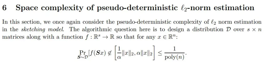
The wrong way of resolving this would be to use delimiter size modifiers, i.e \bigl, \Bigl, \biggl paired with \bigr, \Bigr, \biggr and the like. This is tedious and error-prone, since it will even happily let you match delimiters with different sizes. Indeed, I came across the following formula in a paper recently, where the outer right square brackets was missing and the left one had the wrong size:
The correct way to do this would be to use paired delimiters, which will automatically adjust its size based on its contents, and automatically result in a compile error if the matching right delimiter is not included, or nested at the wrong level. Some of them are given below:
| Raw LaTeX | Rendered |
|---|---|
\left( \frac{1}{x} \right) | \(\left( \frac{1}{x} \right)\) |
\left[ \frac{1}{x} \right] | \(\left[ \frac{1}{x} \right]\) |
\left\{ \frac{1}{x} \right\} | \(\left\{ \frac{1}{x} \right\}\) |
\left\lvert \frac{1}{x} \right\lvert | \(\left\lvert \frac{1}{x} \right\rvert\) |
\left\lceil \frac{1}{x} \right\rceil | \(\left\lceil \frac{1}{x} \right\rceil\) |
In fact, to make things even simpler and more readable, you can declare paired delimiters for use based on the mathtools package, with the following commands due to Ryan O’Donnell:
% Make sure you include \usepackage{mathtools}
\DeclarePairedDelimiter\parens{\lparen}{\rparen}
\DeclarePairedDelimiter\abs{\lvert}{\rvert}
\DeclarePairedDelimiter\norm{\lVert}{\rVert}
\DeclarePairedDelimiter\floor{\lfloor}{\rfloor}
\DeclarePairedDelimiter\ceil{\lceil}{\rceil}
\DeclarePairedDelimiter\braces{\lbrace}{\rbrace}
\DeclarePairedDelimiter\bracks{\lbrack}{\rbrack}
\DeclarePairedDelimiter\angles{\langle}{\rangle}
Then you can now use the custom delimiters as follows, taking note that you need the * for it to auto-resize:
T = \braces*{ \parens*{ x, \sin \frac{1}{x} } : x \in (0, 1] } \cup \braces*{ \parens*{ 0, 0 }}which gives
\[T = \left\{ \left( x, \sin \frac{1}{x} \right) : x \in (0, 1] \right\} \cup \left\{ \left( 0, 0 \right) \right\} \\\]The biggest downside of using custom paired delimiters is having to remember to add the *, otherwise, the delimiters will not auto-resize. This is pretty unfortunate as it still makes it error-prone. There is a proposed solution floating around on StackExchange that relies on a custom command that makes auto-resizing the default, but it’s still a far cry from a parsimonious solution.
Macros for Saving Time and Preventing Mistakes
Macros can be defined using the \newcommand command. The basic syntax is \newcommand{command_name}{command_definition}. For instance, it might get tiring to always type \boldsymbol{A} to refer to a matrix \(\boldsymbol{A}\), so you can use the following macro:
% Macro
\newcommand{\bA}{\boldsymbol{A}}

$$\min_x \lvert \bA x - b \rvert_2^2$$Macros can also take arguments to be substituted within the definition. This is done by adding a [n] argument after your command name, where n is the number of arguments that it should take. You can then reference the positional arguments using #1, #2, and so on. Here, we create a \dotprod macro that takes two arguments:
% Macros
\newcommand{\dotprod}[2]{\langle #1, #2 \rangle}
\newcommand{\bu}{\boldsymbol{u}}
\newcommand{\bv}{\boldsymbol{v}}

$$\left\lvert \dotprod{\bu}{\bv} \right\rvert^2 \leq \dotprod{\bu}{\bu} \cdot \dotprod{\bv}{\bv}$$Macros are incredibly helpful as they help to save time, and ensure that our notation is consistent. However, they can also be used to help to catch mistakes when typesetting grammatically structured things.
For instance, when expressing types and terms in programming language theory, there is often a lot of nested syntactical structure, which could make it easy to make mistakes. Consider the following proof:
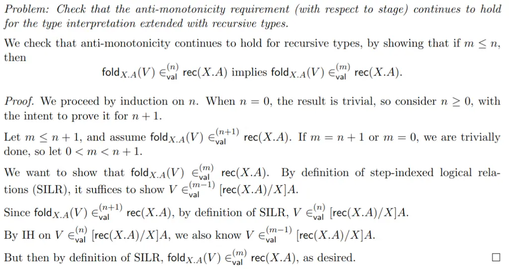
The details are unimportant, but it is clear that it is easy to miss a letter here or a term there in the proof, given how cumbersome the notation is. To avoid this, I used the following macros, due to Robert Harper:
\newcommand{\inval}[2]{\in^{(#1)}_\mathsf{val} #2}
\newcommand{\foldex}[2]{\mathsf{fold}_{#1}(#2)}
\newcommand{\recty}[2]{\mathsf{rec}(#1.#2)}
\newcommand{\Subst}[3]{\sqbracks{{#1}\mathord{/}{#2}}{#3}}
And the source for the proof looks like the following:
We check that anti-monotonicity continues to hold for recursive types,
by showing that if $m \leq n$, then
$$\foldex{X.A}{V} \inval{n}{\recty{X}{A}} \text{ implies } \foldex{X.A}{V} \inval{m}{\recty{X}{A}}. $$

\begin{proof}
We proceed by induction on $n$.
When $n=0$, the result is trivial, so consider $n \geq 0$, with the intent to prove it for $n+1$.

Let $m \leq n + 1$, and assume
$\foldex{X.A}{V} \inval{n+1}{\recty{X}{A}}$. If $m = n + 1$ or $m=0$, we are trivially done, so let $0 < m < n+1$.

We want to show that
$\foldex{X.A}{V} \inval{m}{\recty{X}{A}}$.
By definition of step-indexed logical relations~(SILR), it suffices to show
$V \inval{m-1}{\Subst{\recty{X}{A}}{X}{A}}$.

Since $\foldex{X.A}{V} \inval{n+1}{\recty{X}{A}}$, by definition of SILR,
$V \inval{n}{\Subst{\recty{X}{A}}{X}{A}}$.

By IH on $V \inval{n}{\Subst{\recty{X}{A}}{X}{A}}$,
we also know $V \inval{m-1}{\Subst{\recty{X}{A}}{X}{A}}$.

But then by definition of SILR,
$\foldex{X.A}{V} \inval{m}{\recty{X}{A}}$, as desired. \qedhere
\end{proof}
It is definitely still not the most pleasant thing to read, but at least now you will be less likely to miss an argument or forget to close a parenthesis.
Non-breaking lines
Expressions which are logically a single unit should stay on the same line, instead of being split apart mid-sentence. Cue the following bad example from another paper:
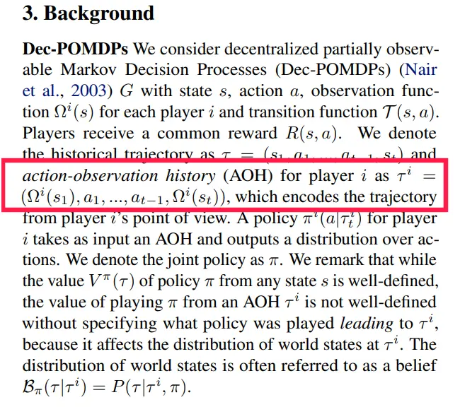
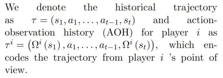
In the area marked in red, we had the expression that was defining \(\tau^i\) get cut in half, which is very jarring visually and interrupts the reader’s train of thought.
To ensure that expressions do not get split, simply wrap it around in curly braces. For instance,
\tau=\left(s_1, a_1, \ldots, a_{t-1}, s_t\right)would be wrapped by { and } on both sides and become
{ \tau=\left(s_1, a_1, \ldots, a_{t-1}, s_t\right) }So if we render the following snippet, which would otherwise have expressions split in half without the wrapped curly braces:
We denote the historical trajectory as
${ \tau=\left(s_1, a_1, \ldots, a_{t-1}, s_t\right) }$
and action-observation history $(\mathrm{AOH})$ for
player $i$ as
${ \tau^i=\left(\Omega^i\left(s_1\right), a_1, \ldots, a_{t-1}, \Omega^i\left(s_t\right)\right) }$,
 which encodes the trajectory from player $i$ 's point of view.
we get the following positive result where there is additional whitespace between the justified text on the first line, to compensate for the expression assigning \(\tau\) to stay on the same line:
Non-breaking space with ~
When referencing figures and equations, you want the text and number (i.e Figure 10) to end up on the same line. This is a negative example, where the region underlined in red shows how it was split up:
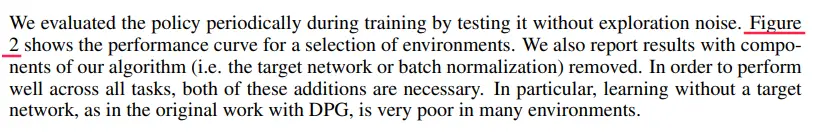
To remedy this, add a ~ after Figure, which LaTeX interprets as a non-breaking space:
We evaluated the policy periodically during training by testing it without exploration noise.
Figure~\ref{fig:env-perf} shows the performance curve for a selection of environments.
This would ensure that “Figure 2” always appears together.
Expressions Should Be Punctuated Like Sentences
Your document is meant to be read, and it should follow the rules and structures of English (or whichever language you are writing in). This means that mathematical expressions should also be punctuated appropriately, which allows it to flow more naturally and make it easier for the reader to follow.
Consider the following example that does not use punctuation:
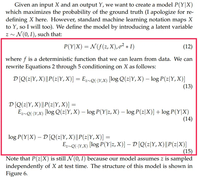
In the region highlighted in red, the expressions do not carry any punctuation at all, and by the end of the last equation (Equation 15), I am almost out of breath trying to process all of the information. In addition, it does not end in a full stop, which does not give me an affordance to take a break mentally until the next paragraph.
Instead, commas should be added after each expression where the expression does not terminate, and the final equation should be ended by a full stop. Here is a good example of punctuation that helps to guide the reader along the author’s train of thought:
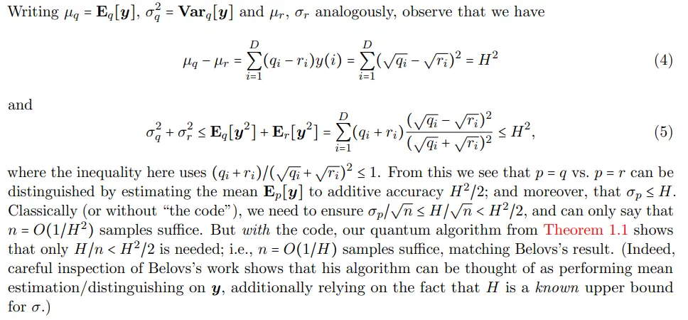
Here is another good example of how using commas for the equations allow the text to flow naturally, where it takes the form of “analogously, observe that we have [foo] and [bar], where the inequality…”:
This even extends to when you pack several equations on a single line, which is common when you are trying to fit the page limit for conference submissions:
The proof environment
The proof environment from the amsthm package is great for signposting to your readers where a proof starts and ends. For instance, consider how it is used in the following example:
\textit{Problem: Show that if $(x_n)_n$ converges to $x$ in the usual sense, then
$\lim_{n \to \infty} x_n = \lim_{\mathcal{F}} x_n$.}

Suppose that $(x_n)_n$ converges to $x$. We show that this $x$ is also the
$\mathcal{F}$-limit of $(x_n)_n$.

\begin{proof}
    Take any $\varepsilon$. Then we know that for some large enough $N$, if $n \geq N$, then
    $x_n \in B_\varepsilon(x)$. Since every non-principal ultrafilter on $\N$ contains
    $\mathcal{F}_\infty$, then $\mathcal{F}$ also contains $ \left\{ n : n \geq N \right\} $,
    since the complement is finite. Therefore since filters are closed upwards, any
    sequence items $x_n$ with $n < N$ that happen to fall in the ball around $x$,
    i.e, $x_n \in B_\varepsilon(x)$
    is also contained in some filter element, so
    $\left\{  n \in \N : \lvert x_n - x \rvert < \varepsilon \right\} \in \mathcal{F}$,
    as desired.
\end{proof}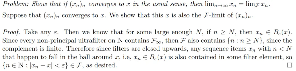
This will helpfully highlight the start of your argument with “Proof”, and terminate it with a square that symbolizes QED.
Terminate Proofs with Explicit \qedhere
Consider the same example as previously, but now you accidentally added an additional newline before the closing \end{proof}, which happens pretty often:
% Same as previously, contents elided for brevity
\begin{proof}
    % Same as previously, contents elided for brevity
    $x_n \in B_\varepsilon(x)$
    is also contained in some filter element, so
    $\left\{  n \in \N : \lvert x_n - x \rvert < \varepsilon \right\} \in \mathcal{F}$,
    as desired.

    % Extra newline here!
\end{proof}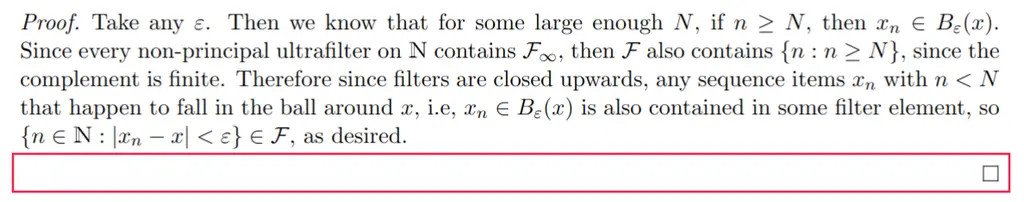
This results in the above scenario, where the QED symbol now appears on the next line by itself, which throws the entire text off-balance visually. To avoid such things happening, always include an explicit \qedhere marker at the end of your proof, which would cause it to always appear on the line that it appears after:
% Same as previously, contents elided for brevity
\begin{proof}
    % Same as previously, contents elided for brevity
    $x_n \in B_\varepsilon(x)$
    is also contained in some filter element, so
    $\left\{  n \in \N : \lvert x_n - x \rvert < \varepsilon \right\} \in \mathcal{F}$,
    as desired. \qedhere % Always add \qedhere once you are done!

    % Extra newline here!
\end{proof}
We would then get the same result as before originally, when we did not have the extra newline.
Spacing
Spacing matters a lot in readability, as it helps to separate logical components. For instance, the following example fails to add spacing before the differential of the variable \(dz\):
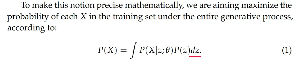
This might seem innocuous, but consider the following example that makes the issue more explicit:
P(X) = \int xyz dxNow we can really see that the quantities are running into each other, and it becomes hard to interpret. Instead, we can add math-mode spacing, summarized in the following table:
| Spacing Expression | Type |
|---|---|
\; | Thick space |
\: | Medium space |
\, | Thin space |
So our new expression now looks like:
P(X) = \int xyz \, dxwhich is much more readable.
align* Environment for Multiline Equations
When using the align* environment, make sure that your ampersands & appear before the symbol that you are aligning against. This ensures that you get the correct spacing.
For instance, the following is wrong, where the & appears after the =:
\begin{align*}
    \nabla_{\mu} (\mathbb{E}_{x\sim q_{\mu}} f(x))  = & \nabla_{\mu} \int_x f(x) q_{\mu}(x) dx                                     \\
                                                    = & \int_x f(x) (\nabla_{\mu} \log q_{\mu}(x))  q_{\mu}(x) dx                  \\
                                                    = & \mathbb{E}_{x \sim q_{\mu}} \left(f(x) \nabla_{\mu} \log q_{\mu}(x)\right)
\end{align*}This is because there is too little spacing after the = sign on each line, which feels very cramped. Putting the & before the = is correct:
\begin{align*}
    \nabla_{\mu} (\mathbb{E}_{x\sim q_{\mu}} f(x)) & = \nabla_{\mu} \int_x f(x) q_{\mu}(x) dx                                     \\
                                                   & =  \int_x f(x) (\nabla_{\mu} \log q_{\mu}(x))  q_{\mu}(x) dx                 \\
                                                   & = \mathbb{E}_{x \sim q_{\mu}} \left(f(x) \nabla_{\mu} \log q_{\mu}(x)\right)
\end{align*}The spacing is much more comfortable now.
Command Mistakes
We now look at some mistakes that arise from using the wrong commands.
Math Operators
Instead of sin (x) \((sin(x))\) or log (x) \((log (x))\), use \sin (x) \((\sin (x))\) and \log (x) \((\log (x))\). The idea extends to many other common math functions. These are math operators that will de-italicize the commands and also take care of the appropriate math-mode spacing between characters:
O(n log n) | \(O(n log n)\) |
O(n \log n) | \(O(n \log n)\) |
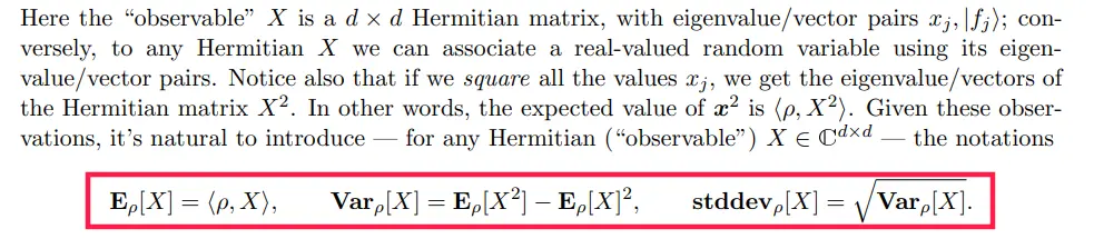
Many times there is a math operator that you need to use repeatedly, but which does not come out of the box. You can define custom math operators with the \DeclareMathOperator command. For instance, here are some commonly used in probability:
\DeclareMathOperator*{\Pr}{\mathbf{Pr}}
\DeclareMathOperator*{\E}{\mathbf{E}}
\DeclareMathOperator*{\Ex}{\mathbf{E}}
\DeclareMathOperator*{\Var}{\mathbf{Var}}
\DeclareMathOperator*{\Cov}{\mathbf{Cov}}
\DeclareMathOperator*{\stddev}{\mathbf{stddev}}
Then you can use it as follows:
\Pr \left[ X \geq a \right] \leq \frac{\Ex[X]}{a}Double quotes
This is more of a rookie mistake since it’s visually very obvious something is wrong. Double quotes don’t work the way you would expect:
\text{"Hello World!"}Instead, surround them in double backticks and single quotes, which is supposed to be reminiscent of the directional strokes of an actual double quote. This allows it to know which side to orient the ticks:
\text{``Hello World!''}
Unfortunately I had to demonstrate this with a screenshot since MathJax only performs math-mode typesetting, but this is an instance of text-mode typesetting.
Epsilons
This is a common mistake due to laziness. Many times, people use \epsilon (\(\epsilon\)) when they really meant to write \varepsilon (\(\varepsilon\)). For instance, in analysis this is usually the case, and therefore writing \epsilon results in a very uncomfortable read:

Using \varepsilon makes the reader feel much more at peace:

Similarly, people tend to get lazy and mix up \phi, \Phi, \varphi (\(\phi, \Phi, \varphi\)), since they are “about the same”. Details matter!
Sets: mathbbm Instead Of mathbb
For sets like \(\mathbb{N}\), you should use \mathbbm{N} (from bbm package) instead of mathbb{N} (from amssymb). See the difference in how the rendering of the set of natural numbers \(\mathbb{N}\) differs, using the same example as the previous section:
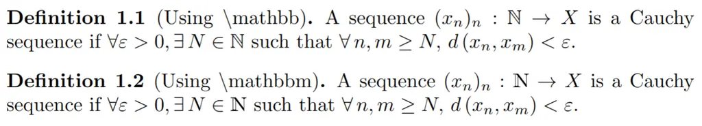
mathbbm causes the symbols to be bolded, which is what you want.
Dots
... and \dots are different. See the difference:
X = \left( X_1, ..., X_n \right)
X = \left( X_1, \dots, X_n \right)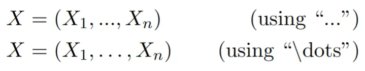
When using “…”, the spacing between each dot, and between the final dot and the comma character is wrong. Always use “\dots”.
Summation and Product
When writing summation or products of terms, use \sum and \prod instead of \Sigma and \Pi. This helps to handle the relative positioning of the limits properly, and is much more idiomatic to read from the raw script:
| Raw LaTeX | Rendered |
|---|---|
\Sigma_{i=1}^n X_i | \(\Sigma_{i=1}^n X_i\) |
\sum_{i=1}^n X_i | \(\sum_{i=1}^n X_i\) |
\Pi_{i=1}^n X_i | \(\Pi_{i=1}^n X_i\) |
\prod_{i=1}^n X_i | \(\prod_{i=1}^n X_i\) |
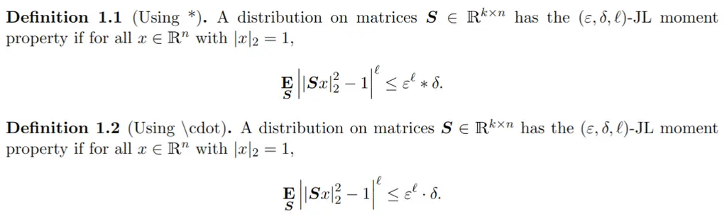
Multiplication
To denote multiplication, use \cdot or times instead of *. See the difference below in the equation:
Mid
For set builder notation or conditional probability, use \mid instead of the pipe |. This helps to handle the spacing between the terms properly:
| Raw LaTeX | Rendered |
|---|---|
p(\mathbf{z}, \mathbf{x}) = p(\mathbf{z}) p(\mathbf{z} | \mathbf{z}) | \(p(\mathbf{z}, \mathbf{x}) = p(\mathbf{z}) p(\mathbf{z} | \mathbf{z})\) |
p(\mathbf{z}, \mathbf{x}) = p(\mathbf{z}) p(\mathbf{z} \mid \mathbf{z}) | \(p(\mathbf{z}, \mathbf{x}) = p(\mathbf{z}) p(\mathbf{z} \mid \mathbf{z})\) |
Angle Brackets
When writing vectors, use the \langle and \rangle instead of the keyboard angle brackets:
| Raw LaTeX | Rendered |
|---|---|
<u, v> | \(<u, v>\) |
\langle u, v \rangle | \(\langle u, v \rangle\) |
Labels
Use \label to label your figures, equations, tables, and so on, and reference them using \ref, instead of hardcoding the number. For instance, \label{fig:myfig} and \ref{fig:myfig}. Including the type of the object in the tag helps to keep track of what it is and ensures that you are referencing it correctly, i.e making sure you write Figure \ref{fig:myfig} instead of accidentally saying something like Table \ref{fig:myfig}.
Conclusion
That was a lot, and I hope it has been a helpful read! I will continue updating this post in the future as and when I feel like there are other important things which should be noted which I missed.
I would like to thank my friend Zack Lee for reviewing this article and for providing valuable suggestions. I would also like to express my thanks to Ryan O’Donnell, and my 15-751 A Theorist’s Toolkit TAs Tim Hsieh and Emre Yolcu for helping me realize a lot of the style-related LaTeX issues mentioned in this post, many of which I made personally in the past.
Related Posts: