$$ \newcommand{\bone}{\mathbf{1}} \newcommand{\bbeta}{\mathbf{\beta}} \newcommand{\bdelta}{\mathbf{\delta}} \newcommand{\bepsilon}{\mathbf{\epsilon}} \newcommand{\blambda}{\mathbf{\lambda}} \newcommand{\bomega}{\mathbf{\omega}} \newcommand{\bpi}{\mathbf{\pi}} \newcommand{\bphi}{\mathbf{\phi}} \newcommand{\bvphi}{\mathbf{\varphi}} \newcommand{\bpsi}{\mathbf{\psi}} \newcommand{\bsigma}{\mathbf{\sigma}} \newcommand{\btheta}{\mathbf{\theta}} \newcommand{\btau}{\mathbf{\tau}} \newcommand{\ba}{\mathbf{a}} \newcommand{\bb}{\mathbf{b}} \newcommand{\bc}{\mathbf{c}} \newcommand{\bd}{\mathbf{d}} \newcommand{\be}{\mathbf{e}} \newcommand{\boldf}{\mathbf{f}} \newcommand{\bg}{\mathbf{g}} \newcommand{\bh}{\mathbf{h}} \newcommand{\bi}{\mathbf{i}} \newcommand{\bj}{\mathbf{j}} \newcommand{\bk}{\mathbf{k}} \newcommand{\bell}{\mathbf{\ell}} \newcommand{\bm}{\mathbf{m}} \newcommand{\bn}{\mathbf{n}} \newcommand{\bo}{\mathbf{o}} \newcommand{\bp}{\mathbf{p}} \newcommand{\bq}{\mathbf{q}} \newcommand{\br}{\mathbf{r}} \newcommand{\bs}{\mathbf{s}} \newcommand{\bt}{\mathbf{t}} \newcommand{\bu}{\mathbf{u}} \newcommand{\bv}{\mathbf{v}} \newcommand{\bw}{\mathbf{w}} \newcommand{\bx}{\mathbf{x}} \newcommand{\by}{\mathbf{y}} \newcommand{\bz}{\mathbf{z}} \newcommand{\bA}{\mathbf{A}} \newcommand{\bB}{\mathbf{B}} \newcommand{\bC}{\mathbf{C}} \newcommand{\bD}{\mathbf{D}} \newcommand{\bE}{\mathbf{E}} \newcommand{\bF}{\mathbf{F}} \newcommand{\bG}{\mathbf{G}} \newcommand{\bH}{\mathbf{H}} \newcommand{\bI}{\mathbf{I}} \newcommand{\bJ}{\mathbf{J}} \newcommand{\bK}{\mathbf{K}} \newcommand{\bL}{\mathbf{L}} \newcommand{\bM}{\mathbf{M}} \newcommand{\bN}{\mathbf{N}} \newcommand{\bP}{\mathbf{P}} \newcommand{\bQ}{\mathbf{Q}} \newcommand{\bR}{\mathbf{R}} \newcommand{\bS}{\mathbf{S}} \newcommand{\bT}{\mathbf{T}} \newcommand{\bU}{\mathbf{U}} \newcommand{\bV}{\mathbf{V}} \newcommand{\bW}{\mathbf{W}} \newcommand{\bX}{\mathbf{X}} \newcommand{\bY}{\mathbf{Y}} \newcommand{\bZ}{\mathbf{Z}} \newcommand{\bsa}{\boldsymbol{a}} \newcommand{\bsb}{\boldsymbol{b}} \newcommand{\bsc}{\boldsymbol{c}} \newcommand{\bsd}{\boldsymbol{d}} \newcommand{\bse}{\boldsymbol{e}} \newcommand{\bsoldf}{\boldsymbol{f}} \newcommand{\bsg}{\boldsymbol{g}} \newcommand{\bsh}{\boldsymbol{h}} \newcommand{\bsi}{\boldsymbol{i}} \newcommand{\bsj}{\boldsymbol{j}} \newcommand{\bsk}{\boldsymbol{k}} \newcommand{\bsell}{\boldsymbol{\ell}} \newcommand{\bsm}{\boldsymbol{m}} \newcommand{\bsn}{\boldsymbol{n}} \newcommand{\bso}{\boldsymbol{o}} \newcommand{\bsp}{\boldsymbol{p}} \newcommand{\bsq}{\boldsymbol{q}} \newcommand{\bsr}{\boldsymbol{r}} \newcommand{\bss}{\boldsymbol{s}} \newcommand{\bst}{\boldsymbol{t}} \newcommand{\bsu}{\boldsymbol{u}} \newcommand{\bsv}{\boldsymbol{v}} \newcommand{\bsw}{\boldsymbol{w}} \newcommand{\bsx}{\boldsymbol{x}} \newcommand{\bsy}{\boldsymbol{y}} \newcommand{\bsz}{\boldsymbol{z}} \newcommand{\bsA}{\boldsymbol{A}} \newcommand{\bsB}{\boldsymbol{B}} \newcommand{\bsC}{\boldsymbol{C}} \newcommand{\bsD}{\boldsymbol{D}} \newcommand{\bsE}{\boldsymbol{E}} \newcommand{\bsF}{\boldsymbol{F}} \newcommand{\bsG}{\boldsymbol{G}} \newcommand{\bsH}{\boldsymbol{H}} \newcommand{\bsI}{\boldsymbol{I}} \newcommand{\bsJ}{\boldsymbol{J}} \newcommand{\bsK}{\boldsymbol{K}} \newcommand{\bsL}{\boldsymbol{L}} \newcommand{\bsM}{\boldsymbol{M}} \newcommand{\bsN}{\boldsymbol{N}} \newcommand{\bsP}{\boldsymbol{P}} \newcommand{\bsQ}{\boldsymbol{Q}} \newcommand{\bsR}{\boldsymbol{R}} \newcommand{\bsS}{\boldsymbol{S}} \newcommand{\bsT}{\boldsymbol{T}} \newcommand{\bsU}{\boldsymbol{U}} \newcommand{\bsV}{\boldsymbol{V}} \newcommand{\bsW}{\boldsymbol{W}} \newcommand{\bsX}{\boldsymbol{X}} \newcommand{\bsY}{\boldsymbol{Y}} \newcommand{\bsZ}{\boldsymbol{Z}} \newcommand{\calA}{\mathcal{A}} \newcommand{\calB}{\mathcal{B}} \newcommand{\calC}{\mathcal{C}} \newcommand{\calD}{\mathcal{D}} \newcommand{\calE}{\mathcal{E}} \newcommand{\calF}{\mathcal{F}} \newcommand{\calG}{\mathcal{G}} \newcommand{\calH}{\mathcal{H}} \newcommand{\calI}{\mathcal{I}} \newcommand{\calJ}{\mathcal{J}} \newcommand{\calK}{\mathcal{K}} \newcommand{\calL}{\mathcal{L}} \newcommand{\calM}{\mathcal{M}} \newcommand{\calN}{\mathcal{N}} \newcommand{\calO}{\mathcal{O}} \newcommand{\calP}{\mathcal{P}} \newcommand{\calQ}{\mathcal{Q}} \newcommand{\calR}{\mathcal{R}} \newcommand{\calS}{\mathcal{S}} \newcommand{\calT}{\mathcal{T}} \newcommand{\calU}{\mathcal{U}} \newcommand{\calV}{\mathcal{V}} \newcommand{\calW}{\mathcal{W}} \newcommand{\calX}{\mathcal{X}} \newcommand{\calY}{\mathcal{Y}} \newcommand{\calZ}{\mathcal{Z}} \newcommand{\R}{\mathbb{R}} \newcommand{\C}{\mathbb{C}} \newcommand{\N}{\mathbb{N}} \newcommand{\Z}{\mathbb{Z}} \newcommand{\F}{\mathbb{F}} \newcommand{\Q}{\mathbb{Q}} \DeclareMathOperator*{\argmax}{arg\,max} \DeclareMathOperator*{\argmin}{arg\,min} \newcommand{\nnz}[1]{\mbox{nnz}(#1)} \newcommand{\dotprod}[2]{\langle #1, #2 \rangle} \newcommand{\ignore}[1]{} \let\Pr\relax \DeclareMathOperator*{\Pr}{\mathbf{Pr}} \newcommand{\E}{\mathbb{E}} \DeclareMathOperator*{\Ex}{\mathbf{E}} \DeclareMathOperator*{\Var}{\mathbf{Var}} \DeclareMathOperator*{\Cov}{\mathbf{Cov}} \DeclareMathOperator*{\stddev}{\mathbf{stddev}} \DeclareMathOperator*{\avg}{avg} \DeclareMathOperator{\poly}{poly} \DeclareMathOperator{\polylog}{polylog} \DeclareMathOperator{\size}{size} \DeclareMathOperator{\sgn}{sgn} \DeclareMathOperator{\dist}{dist} \DeclareMathOperator{\vol}{vol} \DeclareMathOperator{\spn}{span} \DeclareMathOperator{\supp}{supp} \DeclareMathOperator{\tr}{tr} \DeclareMathOperator{\Tr}{Tr} \DeclareMathOperator{\codim}{codim} \DeclareMathOperator{\diag}{diag} \newcommand{\PTIME}{\mathsf{P}} \newcommand{\LOGSPACE}{\mathsf{L}} \newcommand{\ZPP}{\mathsf{ZPP}} \newcommand{\RP}{\mathsf{RP}} \newcommand{\BPP}{\mathsf{BPP}} \newcommand{\P}{\mathsf{P}} \newcommand{\NP}{\mathsf{NP}} \newcommand{\TC}{\mathsf{TC}} \newcommand{\AC}{\mathsf{AC}} \newcommand{\SC}{\mathsf{SC}} \newcommand{\SZK}{\mathsf{SZK}} \newcommand{\AM}{\mathsf{AM}} \newcommand{\IP}{\mathsf{IP}} \newcommand{\PSPACE}{\mathsf{PSPACE}} \newcommand{\EXP}{\mathsf{EXP}} \newcommand{\MIP}{\mathsf{MIP}} \newcommand{\NEXP}{\mathsf{NEXP}} \newcommand{\BQP}{\mathsf{BQP}} \newcommand{\distP}{\mathsf{dist\textbf{P}}} \newcommand{\distNP}{\mathsf{dist\textbf{NP}}} \newcommand{\eps}{\epsilon} \newcommand{\lam}{\lambda} \newcommand{\dleta}{\delta} \newcommand{\simga}{\sigma} \newcommand{\vphi}{\varphi} \newcommand{\la}{\langle} \newcommand{\ra}{\rangle} \newcommand{\wt}[1]{\widetilde{#1}} \newcommand{\wh}[1]{\widehat{#1}} \newcommand{\ol}[1]{\overline{#1}} \newcommand{\ul}[1]{\underline{#1}} \newcommand{\ot}{\otimes} \newcommand{\zo}{\{0,1\}} \newcommand{\co}{:} %\newcommand{\co}{\colon} \newcommand{\bdry}{\partial} \newcommand{\grad}{\nabla} \newcommand{\transp}{^\intercal} \newcommand{\inv}{^{-1}} \newcommand{\symmdiff}{\triangle} \newcommand{\symdiff}{\symmdiff} \newcommand{\half}{\tfrac{1}{2}} \newcommand{\mathbbm}{\Bbb} \newcommand{\bbone}{\mathbbm 1} \newcommand{\Id}{\bbone} \newcommand{\SAT}{\mathsf{SAT}} \newcommand{\bcalG}{\boldsymbol{\calG}} \newcommand{\calbG}{\bcalG} \newcommand{\bcalX}{\boldsymbol{\calX}} \newcommand{\calbX}{\bcalX} \newcommand{\bcalY}{\boldsymbol{\calY}} \newcommand{\calbY}{\bcalY} \newcommand{\bcalZ}{\boldsymbol{\calZ}} \newcommand{\calbZ}{\bcalZ} $$

Solving Genshin Impact's Ancient Azure Stars quest in Linear Time

post.cover
Mona in the event domain, Genshin Impact

It is summer yet again, and miHoYo has blessed us with the Summertime Odyssey event that explores the (often dark and painful) backstories of the cast comprising Kazuha, Xinyan, Fischl, and Mona, back on the setting of the Golden Apple Archipelago.

One puzzle that I found interesting from a computational perspective was a major part of Mona’s questline Ancient Azure Stars, which is the main topic of this post. In this puzzle, you are given a pattern that resembles a constellation that you need to imitate. For readers unfamiliar with Genshin Impact, Mona (pictured in the banner) is an astrologist with the ability to perform divinations, and therefore the idea of forming constellations is very fitting for her character. The puzzle is interesting because even though its mechanics allows for an exponential search space (and also multiple possible solutions), clever algorithmic techniques can speed up finding a valid solution to almost linear time. This post is meant to be accessible to people with only some exposure to algorithms, and takes things step by step.

How the Puzzle Works

The premise is relatively simple: somewhere in the room (perhaps towards the roof), a target constellation is shown, such as the following:

A target constellation to achieve

There are several devices on the ground, initially all inactive, that will project a beam of light when activated, which is achieved by hitting it. These devices can be rotated at discrete intervals corresponding to pointing towards some other device. This means that all devices must be pointing at another device.

Your job is to rotate and activate the right devices such that the pattern formed by the beams corresponds to the desired target constellation. For the previous example, we have the following solution:

A solved configuration of the previous puzzle

The puzzles seem to get progressively harder, with an increasing number of stars in the constellations, and an exponentially growing state space. Or do they?
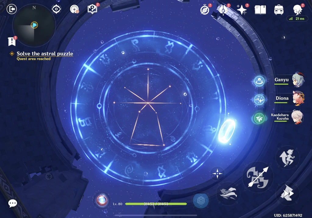
A constellation with many more stars

An Algorithmic Perspective

Let’s make some observations. We can view the problem as forming an unweighted directed graph \(G\) on \(n\) vertices and \(m\) edges, where a beam going from device \(u\) to \(v\) corresponds to a directed edge \((u, v)\) in the graph. Each device can only emit at most one beam, which is when it is activated.

Furthermore, let’s assume that when we treat all directed edges as undirected, the graph is connected (it is possible to reach any vertex from any other vertex). This is admissible since we can just re-run our algorithm later on each individual connected component of the graph. Then we also have that \(n \leq m\).

We know that a tree has \(n-1\) edges and is minimally connected, meaning that the absence of any edge would cause it to be disconnected. Therefore, since \(G\) is connected, there must also be an embedding of a tree \(T\) that forms a subgraph of \(G\) (\(A\) is a subgraph of \(B\) if the vertices and edges of \(A\) form a subset of those of \(B\)) that is also connected.

Let \(C\) be the (connected) constellation that we are trying to form, with \(n_c\) vertices and \(m_c\) edges. Since it is connected, we require \(m_c \geq n_c - 1\).

The Easy Case

If \(m_c = n_c - 1\), then we have a tree, and it is a fact of life that many hard problems are actually very easy on trees (if you are interested, look up the treewidth of a graph, which measures how much a graph is like a tree. The smallest treewidth is 1. Trees have treewidth 1, graphs that can be formed by series and parallel composition have treewidth 2, but the intuition quickly breaks down from here. Many \(\mathsf{NP}\)-hard problems can in fact be solved efficiently on graphs with bounded treewidth!).

We then have a trivial algorithm of just rooting the graph on any vertex, and performing any tree search (say depth-first search) from said vertex, where the reverse of the direction of graph traversal on each edge determines where the beam should go, with the root vertex de-activated. This works because we are essentially pointing the beam of each child vertex towards its parent vertex, and each vertex can only have at most one parent. It takes the optimal \(O(m)\) time.

The Other Case

Otherwise, \(m_c = n_c\). But then the graph is no longer minimally connected, which means that there exists some edge \((u, v)\) where removing \((u, v)\) still causes the resulting graph \(G \setminus (u, v)\) to still be connected as a tree.

Suppose we know what \((u, v)\) is (it does not have to be unique, and in fact is not). Then this makes us really happy, since we can just use the same algorithm as the easy case, but choose vertex \(u\) to be the root, and finally send a beam from \(u\) to \(v\). But how do we find \((u, v)\)?

There is a simple way of doing so by performing depth-first search (DFS) from any arbitrary vertex, making sure to maintain a visited array, where initially all vertices are unvisited except for the root vertex and vertices are marked visited whenever we visit them during DFS. The moment we find that we re-visit a visited vertex \(v\) from some vertex \(u\), we know that we have found \((u, v)\), since it implies that we just found a cycle! This runs in \(O(m)\).

Putting It Together

Taking both steps together, we get an overall \(O(m)\) running time, which is actually also \(O(n)\) given our previous note that \(n \leq m\). This is also the best achievable bound, since we certainly must examine all the inputs which already takes \(O(n)\) time for the algorithm. It certainly looks like Mona will be speeding through these puzzles in no time after all!

Mona looking dapper as always.

Dear readers, let me know if you enjoyed this post in the comments below, and feel free to drop suggestions for future topics!

Copyrights and/or trademarks of any character and/or image used belong to miHoYo.


    Related Posts:

  • Bounding Mixing Times of Markov Chains via the Spectral Gap
  • Notes on 'The Llama 3 Herd of Models'
  • Playing Sound Voltex at Home: Setting Up Unnamed SDVX Clone with the Yuancon SDVX Controller
  • Creating Trackback Requests for Static Sites
  • A Unified Framework for High-Dimensional Analysis of M-Estimators with Decomposable Regularizers: A Guided Walkthrough