Reinforcement Learning Policy Optimization: Deriving the Policy Gradient Update

Reinforcement learning algorithms that learn a policy (as opposed to implicit policy methods like \(\epsilon\)-greedy) optimize their policies by updating their policies in the direction of the gradient. However, the precise environment dynamics are not usually known to us, and the state space is usually also too large to enumerate, which means that we still cannot compute the gradient analytically. In this post, we derive the policy gradient update from scratch, and show how it can be approximated by sampling sufficiently many trajectories.
Optimization Objective
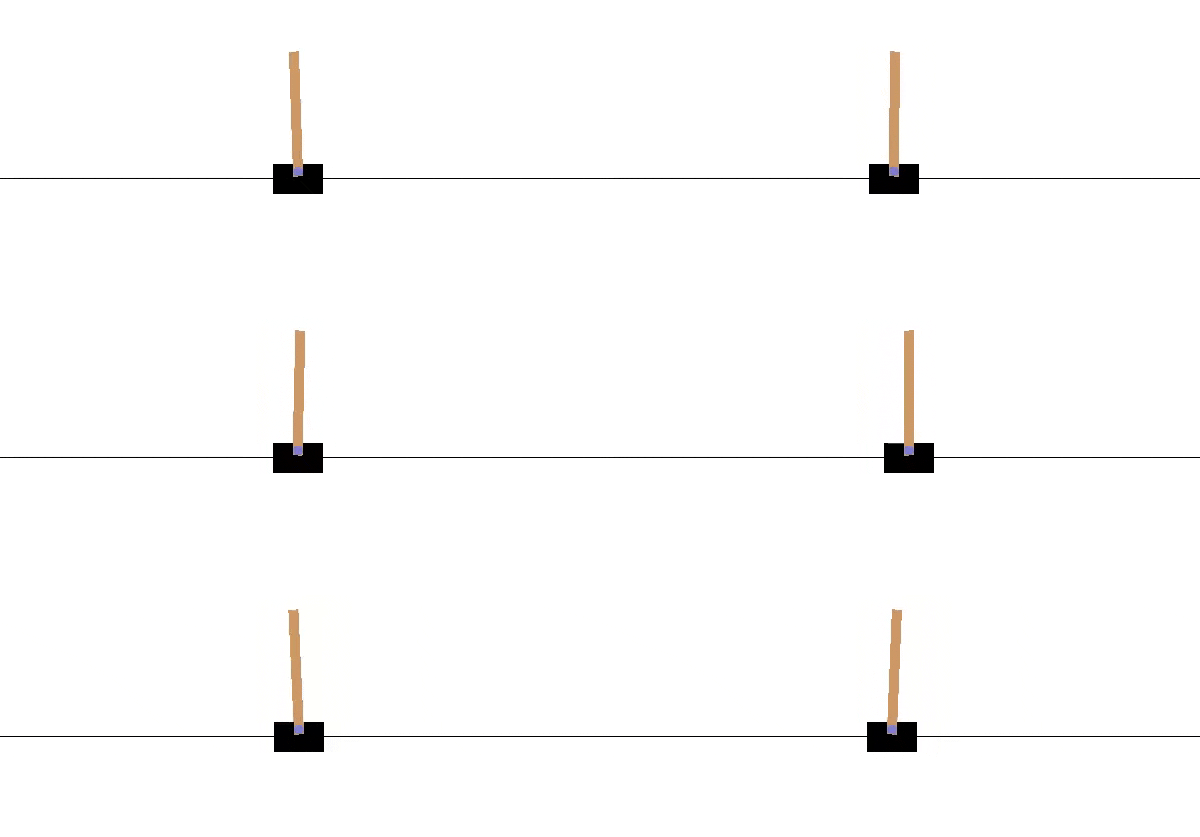
Our goal is to train an agent that is able to maximize its rewards in a given task. For instance, its goal could be to balance a cartpole for as long as possible, where for each time step the pole does not fall down, the agent receives 1 reward, and when the pole falls down the episode is terminated and the agent no longer receives any rewards:

Formally, we want to maximize the expected rewards for our policy over the trajectories that it visits. A trajectory \(\tau\) is defined as state-action pairs \(\tau = (s_0, a_0, s_1, a_1, \dots, s_H, a_H, s_{H+1})\), where \(H\) is horizon of the trajectory, i.e the duration until the episode is terminated, and \(s_t, a_t\) are the states and actions performed at each time step \(t\).
This can be formalized as the following objective:
\[\begin{align} & \max_\theta \mathbb{E}_{\tau \sim P_\theta(\tau)} [R(\tau)] \\ = & \max_\theta \sum\limits_\tau P_\theta(\tau) R(\tau) \\ = & \max_\theta U(\theta), \end{align}\]where \(\tau\) refers to a trajectory of state-action pairs, \(P_\theta(\tau)\) denotes the probability of experiencing trajectory \(\tau\) under policy \(\theta\), and \(R(\tau)\) is the reward under trajectory \(\tau\), and \(U(\theta)\) is shorthand for the expression for brevity.
The probability of \(P_\theta(\tau)\) is given by the following:
\[\begin{align} P_\theta(\tau) = \prod_{t=0}^H P(s_{t+1} \mid s_t, a_t) \cdot \pi_\theta (a_t \mid s_t), \end{align}\]where in words, it is the product over each time step \(t\), of the probability of taking the action at time \(t\) in the trajectory \(a_t\) when we were in state \(s_t\) under our policy \(\pi_\theta\), given by \(\pi_\theta(a_t \mid s_t)\), multiplied by the probability that the environment transitions us from \(s_t\) to \(s_{t+1}\) given that we performed action \(a_t\). Note that we do not necessarily know this environment transition probability \(P(s_{t+1} \mid s_t, a_t)\).
Deriving the Gradient Update
To perform a gradient-based update on \(\theta\) to increase the reward, we need to compute the derivative with respect to our policy \(\theta\), i.e \(\nabla_\theta \mathbb{E}_{\tau \sim P(\tau; \theta)} [R(\tau)]\). Let’s walk through the derivation step by step:
\[\begin{align*} \nabla_\theta \mathbb{E}_{\tau \sim P_\theta(\tau)} [R(\tau)] & = \nabla_\theta \sum\limits_\tau P_\theta(\tau) R(\tau) \\ & = \sum\limits_\tau \nabla_\theta P_\theta(\tau) R(\tau) & \text{(uh oh...)}\\ \end{align*}\]It appears that we are already stuck here, since \(\nabla_\theta P_\theta(\tau)\) will result in many repeated applications of the chain rule since \(P_\theta(\tau)\) is a huge product containing our policy transition probabilities, and will quickly get out of hand to be computed feasibly.
Instead, the trick is to multiply by 1 on the left:
\[\begin{align*} \sum\limits_\tau \nabla_\theta P_\theta(\tau) R(\tau) &= \sum\limits_\tau \frac{ P_\theta(\tau) }{ P_\theta(\tau) } \nabla_\theta P_\theta(\tau) R(\tau) & \text{(multiplying by 1)} \\ &= \sum\limits_\tau P_\theta(\tau) \frac{ \nabla_\theta P_\theta(\tau) }{ P_\theta(\tau) } R(\tau) & \text{(rearranging)} \\ &= \sum\limits_\tau P_\theta(\tau) \nabla_\theta \log P_\theta(\tau) R(\tau) & \text{($\frac{d}{dx} \log f(x) = \frac{f'(x)}{f(x)} $)} \\ &= \mathbb{E}_{\tau \sim P_\theta(\tau)} \left[ \nabla_\theta \log P_\theta(\tau) R(\tau) \right] \\ &\approx \frac{1}{N} \sum\limits_{i=1}^N \nabla_\theta \log P_\theta(\tau_i) R(\tau_i), \\ \end{align*}\]where we can use \(\frac{1}{N} \sum\limits_{i=1}^N \nabla_\theta \log P_\theta(\tau_i) R(\tau_i)\) as our estimator, which converges to the true expectation as our number of trajectory samples \(N\) increases.
We can compute \(\nabla_\theta \log P_\theta(\tau_i)\) for each sampled trajectory \(\tau_i\), and then take their average. This can be done as follows:
\[\begin{align*} \nabla_\theta \log P_\theta(\tau_i) & = \nabla_\theta \log P_\theta(s_0, a_0, \dots, s_H, a_H, s_{H+1}) \\ & = \nabla_\theta \log \left[ \prod_{t=0}^H P(s_{t+1} \mid s_t, a_t) \cdot \pi_\theta (a_t \mid s_t), \right] \\ & = \nabla_\theta \left[ \sum\limits_{t=0}^H \log P(s_{t+1} \mid s_t, a_t) + \log \pi_\theta (a_t \mid s_t) \right] \\ & = \nabla_\theta \sum\limits_{t=0}^H \log \pi_\theta (a_t \mid s_t) \\ & \qquad \qquad \text{(first term does not depend on $\theta$, becomes zero)} \\ & = \sum\limits_{t=0}^H \nabla_\theta \log \pi_\theta (a_t \mid s_t),\\ \end{align*}\]where the last expression is easily computable for models such as neural networks since it is end-to-end differentiable.
With the approximate gradient \(\nabla_\theta U(\theta)\) in hand, we can now perform our policy gradient update as
\[\begin{align*} \theta_{\mbox{new}} = \theta_{\mbox{old}} + \alpha \nabla_\theta U(\theta), \end{align*}\]for some choice of step size \(\alpha\).
Takeaways
In this post, we saw from first principles how taking the gradients of many sampled trajectories does indeed converge to the true policy gradient.
This method of multiplying by 1 to pull out a probability term so that a summation can be converted into an expectation is widely used in machine learning, such as for computing variational autoencoder (VAE) loss. It is known as the log derivative trick.
The estimator \(\frac{1}{N} \sum\limits_{i=1}^N \nabla_\theta \log P_\theta(\tau_i) R(\tau_i)\) is also sometimes known as the REINFORCE estimator, after the popular REINFORCE algorithm.
One limitation of this approach is that it requires \(\pi_\theta\) to be differentiable. However, given how most RL models rely on neural networks, this is not a significant restriction.
Choosing the right step size \(\alpha\) is actually not straightforward. It is different from the offline supervised-learning context, where you can use methods like AdaGrad or RMSProp which adaptively chooses a learning rate for you, and even if the learning rate was not optimal it just takes more iterations to converge. On the other hand, in reinforcement learning, a learning rate that is too small results in inefficient use of trajectory samples as they cannot be trivially re-used since it depends on your current policy, and a learning rate that is too large can result in the policy becoming bad, which is difficult to recover from since future trajectories would also become bad.
We will discuss three important methods to choose an appropriate step size in a future post: Natural Policy Gradients, Proximal Policy Optimization (PPO), and Trust Region Policy Optimization (TRPO). Hope to see you around!
I would like to express my thanks to my friend Jun Yu Tan for reviewing this article and for providing valuable suggestions.
References
Related Posts: