Writing a DPLL SAT Solver

Boolean satisfiability (SAT) solvers have played an important role in software and hardware verification, automatic test pattern generation, planning, scheduling, and solving challenging problems in algebra.
In this post, I talk about my experience writing my own SAT solver, its implementation details, designs and algorithms used, some comparisons between using different heuristics for splitting and choosing of variable assignments in the unforced case, challenges faced, and possible future directions.
You can find the code for the project on Github here.
Overview
My SAT solver uses the classical Davis–Putnam–Logemann–Loveland (DPLL) algorithm, which is based off backtracking search. In order to speed up the search process, unit propagation (also known as boolean constraint propagation), and the usage of watchlists for ease of backtracking is also implemented.
Trying it out
You can skip this section if you don’t intend to run the SAT solver and just want to learn more about how it is implemented.
To run the SAT solver, run ./src/sat.py <filename>. It also takes in verbosity flags, -v and -vv depending on the level desired. By default, only the test case being run and the result is given as output. -v prints the initial SAT formula, the current decisions being made and whenever backtracking is performed. It also outputs the final satisfying assignment. For instance, try running ./src/sat.py -v dat/sat/uf50-0100.cnf to see the assignments for one of the test cases. -vv outputs almost all information about what the algorithm is currently doing.
As an example, try running ./src/sat.py small/small-sat1.cnf, which corresponds to the CNF \((x_1 \vee x_2 \vee x_3) \wedge (\neg x_1 \vee \neg x_2 \vee \neg x_3)\), which should output \(\texttt{SATISFIABLE}\). For an unsatisfiable instance, try running ./src/sat.py small/small-unsat2.cnf, which is an unsatisfiable instance corresponding to the following SAT instance:
This should output \(\texttt{UNSATISFIABLE}\).
Algorithms
The two interesting algorithms implemented for SAT solving are DPLL and unit propagation. The DPLL forms the main logic of assigning variables and performing backtracking and re-assignment if conflict arise. Unit propagation is an optimization that helps us prune our search space and converge to a solution if any faster. We examine both in detail.
DPLL
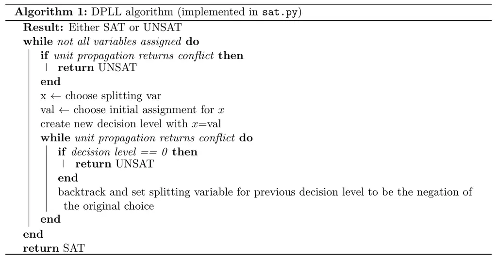
The DPLL algorithm works as follows: at every step, it chooses a variable to assign, and also chooses what value to first try assigning it. Whenever it makes such a voluntary assignment (i.e not forced), a new decision level is created. A decision level contains all the current assignments, and the variable that created the decision level. In our code, this is handled by the \(\texttt{Assignment}\) class, and the \(\texttt{assignment_stack}\) keeps track of the decision levels.
Once a new decision level is created, we perform unit propagation (elaborated next). Unit propagation forces assignments, so there is no need to create new decision levels. If unit propagation results in conflicts (i.e a clause that is unsatisfiable for sure given the current assignments), we need to backtrack. Backtracking involves returning to the previous decision level, and forcing the assignment of the variable that caused the conflicting decision level to the negation of its previous assignment. If we ever run out of decision levels, it means that all possible choices of assignments results in conflicts, and therefore the SAT instance is unsatisfiable. By using decision levels (and also watchlists, elaborated later), we can write our code in an iterative instead of recursive manner, which is significantly faster as it avoids the overhead of moving around stack frames.
In the DPLL algorithm, we allow the user to specify their own heuristics for both choosing the splitting variable, and the initial first assignment to use. This can be done by modifying \(\texttt{choose_splitting_var}\) and \(\texttt{choose_assn}\) in \(\texttt{heuristics.py}\) respectively. The file is well-documented and contains information on the information that is passed in that can be used to write a useful heuristic.
By default, if either function throws \(\texttt{NotImplementedError}\), the SAT solver will choose the first unassigned variable, and default to trying to assign it to true first. The sample implementation given in \(\texttt{heuristics.py}\) uses a randomized strategy for both \(\texttt{choose_splitting_var}\) and \(\texttt{choose_assn}\), and is meant to demonstrate how the arguments can be used.
Unit Propagation
The idea behind unit propagation is that when we have all other vars in a clause evaluating to false except one, then the final one must be set such that it evaluates to true. This is a forced assignment. This allows for great speedups as the search space can be drastically reduced.
Instead of naively inspecting every clause during unit propagation which is costly, we can instead only examine clauses that are actually affected by assignments. In particular, we only care about clauses that contains vars whose corresponding variables are assigned a value that makes it evaluate to false. For instance, in the clause \((x_1 \vee x_2 \vee x_3)\) we can continue to sleep peacefully \(x_1\) was assigned to true, but we definitely will be concerned if \(x_1\) was assigned to be false.
To this end, we introduce the idea of watched literals introduced by Moskewicz et al. Each clause contains a watchlist, which contains two variables that it is currently watching. It is initialized to be the first two variables. The requirements are that we must always have at least one of the variables that it is watching be non-false (i.e either true or unknown). Whenever this is violated, the clause must find another variable to watch. If this is not possible, then unit propagation returns \(\texttt{CONFLICT}\).
Another benefit of using watched literals is that during backtracking, our constraints can only be relaxed (i.e our variables can be unassigned but never assigned), and therefore we do not need to update them.
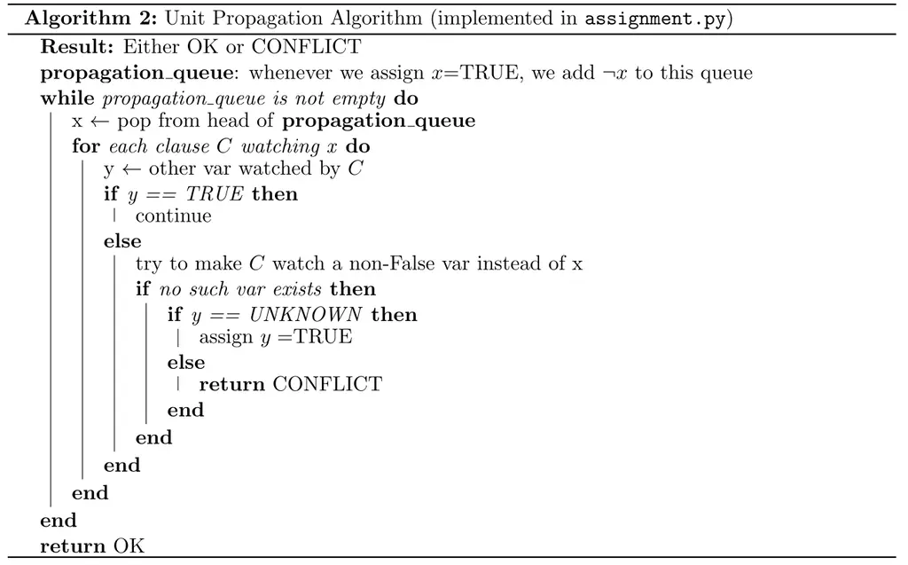
In the unit propagation algorithm given above, we go through each of the vars that is now false as a result of previous assignments, and look at all the clauses watching them, and try to maintain the invariant that each clause is watching at least one non-False variable. If this is not possible and the other variable \(y\) being watched is an unknown, we then know we can force it to be true. If \(y\) is already assigned, then we have a conflict, and backtracking is inevitable.
Experiments with various Heuristics
The SAT solving framework provides flexibility for changing the heuristics used easily. I ran some tests to see how well they performed relative to each other, with three different strategies:
- Default strategy: use first unassigned variable, and always assign True first
- Randomized strategy: use any unassigned variable, and use random initial truth values
- Majority strategy: use first unassigned variable, and assign it the value that will satisfy the majority of the clauses that it appears in
The results are given below:
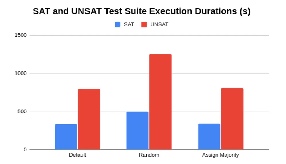
It is surprising that the random strategy runs much slower than the default strategy and the majority strategy. It is also surprising that the default naive strategy actually performs the best in this case, even though intuitively the majority strategy should perform better. A possible explanation for this behavior is that the majority strategy is a greedy strategy, and therefore random SAT instances could be resistant to greedy strategies.
Future Directions
There are many other promising optimizations that can be added to improve the speed of this SAT solver.
One possibility is to implement conflict-driven clause learning (CDCL) introduced by Marques et al, which is an extension of DPLL where it remembers conflicts that occurred previously and uses that to learn new clauses. This helps to prune the search space. We can also consider extending CDCL with random restarts, which has shown good results in practice. Random restarts has been shown to allow CDCL to learn about persistently troublesome conflicting variables earlier, and therefore converges to a solution faster.
Another direction is to improve our heuristics for choosing variables and their values. MOMS (Maximum Occurence in clauses of Minimum Size) is a heuristic where we prioritize assigning variables that occurs the highest number of times in short clauses. Bohm’s heuristic chooses the variable that appears the most in unsatisfied clauses. The VSIDS (Variable State Independent Decaying Sum) heuristic assigns each variable a weight, which is decayed at each time step. The weight of a variable is increased whenever it is involved in a conflicting clause. The heuristic then selects the variable with the highest score.
Other directions include using conflict-directed backjumping, which allows the solver to go more than one level up the decision level given certain conditions. Backjumping is a general technique used to speed up backtracking algorithms.
Running Test Cases
You can skip this section unless you are playing around with the code. Running make setup will generate the testcases directory. The testcases are taken from SATLIB, and are split into two folders - dat/sat and dat/unsat, for satisfiable and unsatisfiable instances respectively. Each directory contains 1000 SAT instances, each of which contains 50 variable and 218 clauses. SATLIB claims that these instances are generated uniform at random.
To run the SAT solver on all the instances that should be satisfiable, run make sat. This will take a while (around 10 minutes). To run unsatisfiable instances, run make unsat. This will take even longer.
Closing Thoughts
Writing the SAT sovler was a fun adventure. Maintaining the watched literals for each clause correctly was much trickier than I expected, and I had to write a few debugging routines and put assertions to diagnose and fix a few bugs (see check_invariants in sat.py). Debugging was also challenging because the SAT solver always performed correctly on my small hand-crafted SAT instances, and only failed on the much larger testcases from SATLIB which is far more difficult to trace. It also took me a while to initially convince myself of the correctness of the algorithm from the interplay between the propagation queue, the watched literals, and the decision levels, even though it seems completely obvious to me now.
I hope you’ve found this post interesting and learned a thing or two. Let me know what you think in the comments!
References
- Frank Van Harmelen, Vladimir Lifschitz, and Bruce Porter. Handbook of knowledge representation. Elsevier, 2010.
- Jediah Katz. Algorithms for SAT.
- Swords. Basics of SAT Solving Algorithms, Dec 2008.
- M.w. Moskewicz, C.f. Madigan, Y. Zhao, L. Zhang, and S. Malik. Chaff: Engineering an Efficient SAT Solver. Proceedings of the 38th Design Automation Conference (IEEE Cat. No.01CH37232).
- Handbook of satisfiability. IOS Press, 2009.
- Carla Gomes, Bart Selman, and Henry Kautz. Boosting combinatorial search through randomization. Proceedings of the National Conference on Artificial Intelligence, 03 2003.
- Richard M. Stallman and Gerald J. Sussman. Forward reasoning and dependency-directed backtracking in a system for computer-aided circuit analysis. Artificial Intelligence, 9(2):135–196, 1977
Related Posts: