Three Important Things
1. Diffusion-LM Setup
This was an influential paper for being the first one to introduce how we can train text diffusion models in a continuous latent space. Previous text diffusion models are trained in a discrete space, where words/tokens are refined by either permutation and/or masking.

Train such a model begins by first embedding each word in the sequence, which is a stochastic process:
\[q_\phi\left(\mathbf{x}_0 \mid \mathbf{w}\right)=\mathcal{N}\left(\operatorname{EmB}(\mathbf{w}), \sigma_0 I\right)\]One question I had when reading this was why the embedding had to be stochastic, but it was not really explained in the paper. Perhaps it is trying to make the embedding step also somewhat like a noising/denoising process like the rest of it?
After embedding $\mathbf{w}$, we now get a continuous latent $\mathbf{x}_0$ which represents the clean data. This goes through the standard diffusion model noising/denoising steps.
Finally, when the corrupted data is denoised back to $\mathbf{x}_0$, they added a rounding step to round/unembed it back to the closest word vector, where it is sampled with a softmax.
The training loss objective is a mix of the standard diffusion denoising loss, encouraging the embeddings to be close to the predictions for the last step $\mathbf{x}_0$, and maximizing the likelihood of the data:
\[\mathcal{L}_{\text {simple }}^{\mathrm{e} 2 \mathrm{e}}(\mathbf{w})=\underset{q_\phi\left(\mathbf{x}_{0: T} \mid \mathbf{w}\right)}{\mathbb{E}}\left[\mathcal{L}_{\text {simple }}\left(\mathbf{x}_0\right)+\left\|\operatorname{EMB}(\mathbf{w})-\mu_\theta\left(\mathbf{x}_1, 1\right)\right\|^2-\log p_\theta\left(\mathbf{w} \mid \mathbf{x}_0\right)\right]\]2. Reducing Rounding Errors
One issue they found is that since the loss only enforces that the latents at the last step is close to the embeddings, the model is often in a superposition state and doesn’t really want to commit to any word, meaning that there’s no single word that has high probability. For instance, it may think of producing both “I want a dog” and “A cat is nice”, but end up sampling “I cat a nice” which doesn’t make sense.
This means that during sampling, it is possible for nonsensical outputs to be produced since there is a lack of consistency between the sampled words in the sequence.
To fix this, they modified the objective such that the model is also encouraged to predict the denoised latent $\mathbf{x}_0$ at each step of the denoising process, which encourages it to commit to an embedding early.
In addition, they used what they coined the “clamping trick” during inference - at each denoising step, they clamp the current latent $\mathbf{x}_t$ to the closest word embedding to further force it to commit to a word, ensuring that the overall generation is now more consistent.
3. Controllable Text Generation
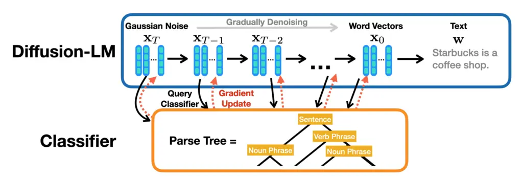
Control generation is done by using a trained classifier to guide the denoising process through the latens. This is done by adding an additional gradient step in the direction of the classifier at each step.
Most Glaring Deficiency
Experiments were pretty small scale and on datasets/tasks that are quite synthetic. The need for a classifier also makes this harder to steer as opposed to prompting approaches in traditional autoregressive LMs.
Conclusions for Future Work
This work provides the foundation on how we can move from a discrete text to continuous latent space, which opens up many interesting directions for advancing language diffusion models.