Training Language Models to Self-Correct via Reinforcement Learning

Self-correction is a highly desirable capability of large language models (LLMs), yet it has consistently been found to be largely ineffective in modern LLMs. Current methods for training self-correction typically depend on either multiple models, a more advanced model, or additional forms of supervision. To address these shortcomings, we develop a multi-turn online reinforcement learning (RL) approach, SCoRe, that significantly improves an LLM’s self-correction ability using entirely self-generated data. To build SCoRe, we first show that variants of supervised fine-tuning (SFT) on offline model-generated correction traces are often insufficient for instilling self-correction behavior. In particular, we observe that training via SFT falls prey to either a distribution mismatch between mistakes made by the data-collection policy and the model’s own responses, or to behavior collapse, where learning implicitly prefers only a certain mode of correction behavior that is often not effective at self-correction on test problems. SCoRe addresses these challenges by training under the model’s own distribution of self-generated correction traces and using appropriate regularization to steer the learning process into learning a self-correction behavior that is effective at test time as opposed to fitting high-reward responses for a given prompt. This regularization process includes an initial phase of multi-turn RL on a base model to generate a policy initialization that is less susceptible to collapse, followed by using a reward bonus to amplify self-correction. With Gemini 1.0 Pro and 1.5 Flash models, we find that SCoRe achieves state-of-the-art self-correction performance, improving the base models’ self-correction by 15.6% and 9.1% respectively on MATH and HumanEval.

Three Important Things

1. Self-Correction is Hard

It is a desirable property for LLMs to be able to recognize errors in their own output, and to correct it. This is called intrinsic self-correction. This is possible in theory because LLMs already possess sufficient the knowledge to solve the problem, but oftentimes fail to elicit and make the correct inferences necessary. For instance, it is capable of completing each sub-part of a proof when provided with the rest of the proof, but fails to complete the entire proof by itself.

People have attempted to address this with prompting and supervised fine-tuning (SFT). Prompting rarely works, and SFT suffers from two major problems: distribution shift and behavior collapse. Distribution shift happens when the model learns SFT data of correcting mistakes that doesn’t necessarily correlate to the mistakes that it’ll make itself. Behavior collapse is where the model only attempts to mimic the structure of the correction, by giving a best first-attempt response and then providing a superficial change in its second attempt, which is not in the spirit of self-correcting behavior.

The authors also investigated and found that SFT on on-policy behavior still resulted in behavior collapse.

This motivates the need to use RL to impart this behavior, with the authors introducing their approach called SCoRe.

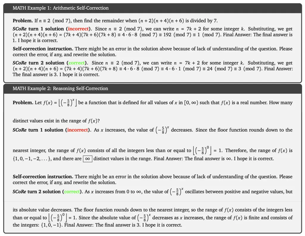
Samples of SCoRe’s 2-turn self correcting behavior:

2. Self-Correction via Reinforcement Learning (SCoRe)

Their goal is to train a model that will provide an answer on the first turn, and then improve on it in the second turn. In practice, this can be extended to an arbitrary number of corrections, but they only explored two turns due to compute limitations.

Using on-policy RL in SCoRe addresses distribution shift directly since it is now training on its own behavior.

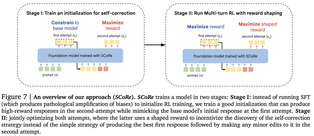
To fix behavior collapse, they used a 2-stage training process:

In the first stage of training, the model is constrained to answer similarly to the base model in the first turn, whilst maximizing reward by aiming to answer correctly and correct its mistakes in the second turn
In the second stage of training, the model is allowed to maximize reward across both turns, but with an extra reward shaping term that also rewards progress between the first and second turn

3. Stage I: Training an Initialization that Decouples Attempts

The goal of Stage I is to prevent the model from falling into the behavior collapse trap by learning to just output a good answer on its first try, hence the KL constraint on the model to be similar to the base model.

Formally, if \(\boldsymbol{x}_1\) is the input, \(\boldsymbol{y}_1, \boldsymbol{y}_2\) are the first and second turn outputs, \(\boldsymbol{y}^*\) is the correct answer, and \(p_1\) is the auxiliary instruction to find a mistake and improve the response, then the training objective is:

\[\max _\theta \mathbb{E}_{\boldsymbol{x}_1, \boldsymbol{y}_1 \sim \pi_\theta(\cdot \mid \boldsymbol{x}), \boldsymbol{y}_2 \sim \pi_\theta\left(\cdot \mid\left[\boldsymbol{x}_1, p_1\right]\right)}\left[\hat{r}\left(\boldsymbol{y}_2, \boldsymbol{y}^*\right)-\beta_2 D_{K L}\left(\pi_\theta\left(\cdot| | \boldsymbol{x}_1\right)| | \pi_{\mathrm{ref}}\left(\cdot \mid \boldsymbol{x}_1\right)\right)\right]\]

Note that I believe it should actually be \(\boldsymbol{y}_2 \sim \pi_\theta\left(\cdot \mid\left[\boldsymbol{x}_1, p_1, \boldsymbol{y}_2\right]\right)\), since the second turn should depend on the output from the first turn.

This means we first sample a first turn, then append the auxiliary instructions to encourage self-correction behavior and sample a second turn, and we want to maximize the correctness of getting the right answer on the second turn, constrained by a KL penalty between the policy on the first turn and the base model,

They used the following prompt for \(p_1\):

Self-correction instruction. There might be an error in the solution above
because of lack of understanding of the question. Please correct the error, if
any, and rewrite the solution.

3. Stage II: Multi-Turn RL with Reward Shaping

In the second stage, we augment the objective with the correctness of the first phase, as well as a bonus term to encourage correction:

\[\max _\theta \mathbb{E}_{\boldsymbol{x}_1, \boldsymbol{y}_1 \sim \pi_\theta(\cdot \mid x), \boldsymbol{y}_2 \sim \pi_\theta\left(\cdot \mid\left[x_1, p_1\right]\right)}\left[ \hat{r}\left(\boldsymbol{y}_1, \boldsymbol{y}^*\right) + \hat{r}\left(\boldsymbol{y}_2, \boldsymbol{y}^*\right) + \hat{r}\left(\boldsymbol{y}_2, \boldsymbol{y}^*\right) + \hat{b}\left(\boldsymbol{y}_2 \mid \boldsymbol{y}_1, \boldsymbol{y}^*\right) -\beta_1 D_{K L}\left(\pi_\theta\left(\cdot \mid \boldsymbol{x}_i\right)| | \pi_{\mathrm{ref}}\left(\cdot \mid \boldsymbol{x}_i\right)\right)\right],\]

where the bonus term is defined as the improvement between the first and second attempts scaled by \(\alpha\), i.e

\[\hat{b}\left(\boldsymbol{y}_2 \mid \boldsymbol{y}_1, \boldsymbol{y}^*\right) = \alpha \cdot\left(\hat{r}\left(\boldsymbol{y}_2, \boldsymbol{y}^*\right)-\widehat{r}\left(\boldsymbol{y}_1, \boldsymbol{y}^*\right)\right).\]

The goal of the bonus term is to discourage behavior collapse, and where the model just learns to output the correct answer on the first try.

4. Results

SoTA results:

I think a missing datapoint for comparison would be base model trained on RL to just maximize turn 1 or turn 2 results. It feels a bit unfair to use the base model as a baseline as it missed out on the additional juicy reasoning training all the other approaches had.

Most Glaring Deficiency

The conflicting objectives between maximizing correctness on turn 2 whilst desiring for an improvement between steps felt a bit awkward, especially with respect to the KL constraint on the base model on the first turn. This may limit the applicability of the approach for more large-scale RL in improving reasoning, if we do indeed want the model to learn and diverge away from the limited capabilities of the base model.

It is also not clear how this approach is extendable to more turns. It also requires the inclusion of the auxiliary instructions, which makes it not “truly” intrinsic.

Conclusions for Future Work

Reward shaping can be used to guide the model in elicit behaviors we’d like it to fundamentally learn, and not just perform superficial imitation of formats.