Reconciling modern machine learning practice and the bias-variance trade-off

Breakthroughs in machine learning are rapidly changing science and society, yet our fundamental understanding of this technology has lagged far behind. Indeed, one of the central tenets of the field, the bias-variance trade-off, appears to be at odds with the observed behavior of methods used in the modern machine learning practice. The bias-variance trade-off implies that a model should balance under-fitting and over-fitting: rich enough to express underlying structure in data, simple enough to avoid fitting spurious patterns. However, in the modern practice, very rich models such as neural networks are trained to exactly fit (i.e., interpolate) the data. Classically, such models would be considered over-fit, and yet they often obtain high accuracy on test data. This apparent contradiction has raised questions about the mathematical foundations of machine learning and their relevance to practitioners. In this paper, we reconcile the classical understanding and the modern practice within a unified performance curve. This "double descent" curve subsumes the textbook U-shaped bias-variance trade-off curve by showing how increasing model capacity beyond the point of interpolation results in improved performance. We provide evidence for the existence and ubiquity of double descent for a wide spectrum of models and datasets, and we posit a mechanism for its emergence. This connection between the performance and the structure of machine learning models delineates the limits of classical analyses, and has implications for both the theory and practice of machine learning.

Three Important Things

1. Double Descent

This was the paper that introduced “double descent”, which shows that the U-shaped bias-variance tradeoff curve in classical statistics is actually incomplete, and that increasing model capacity beyond the interpolation threshold (i.e where training error goes to 0) can cause test loss to go even lower than the minima from the under-parameterized regime.

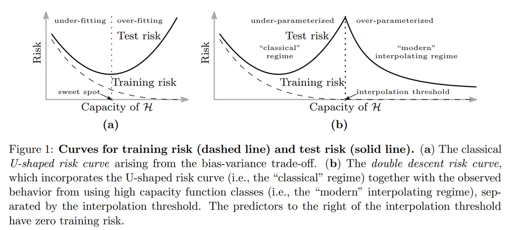
They postulated the reason why this was not observed earlier was due to the following:

It requires a parametric function class that can scale to arbitrary complexity, but classical statistics usually works with a small, fixed set of features
Regularization is often performed, which can prevent interpolation and hence mask the interpolation peak
Computational benefits of kernel methods only hold when the number of datapoints is larger than model capacity, hence this over-parameterized regime was overlooked
Early stopping is commonly employed and also prevents observing this phenomenon

2. Observations on NNs with RFFs, Decision Trees, and Ensemble Methods

They noted double descent on neural networks parameterized by an equivalent Random Fourier Feature model, decision trees, as well as ensemble methods. I’ll just focus on the results for the RFF case.

In RFF, a model family $\mathcal{H}_N$ parameterized by $N$ complex-valued parameters (via $a_k, v_k$) is given by

\[h(x)=\sum_{k=1}^N a_k \phi\left(x ; v_k\right) \quad \text{ where }\quad \phi(x ; v):=e^{\sqrt{-1}\langle v, x\rangle}\]

During training, the optimal parameters are found by ERM. When solutions are not unique, the coefficients $(a_1, \cdots, a_N)$ with the smallest $\ell_2$ norm is chosen.

Thus we can see that increasing $N$ makes the function class more expressive, and in fact when you take $n \to \infty$ this converges to the Reproducing Kernel Hilbert Space.

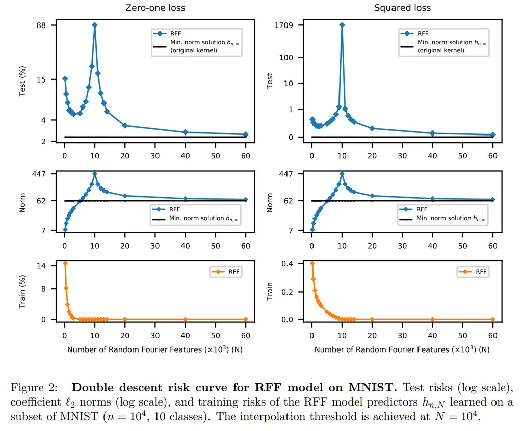
It was interesting that the interpolation threshold corresponds to the number of training datapoints. We also see that the norm also increases as more functions are available to attempt to interpolate the datapoints, where it peaks at the interpolation threshold, before tapering off and converging to the minimum norm solution with the Gaussian kernel for RKHS.

3. Approximation Theorem

They provided some theoretical justification on why choosing the minimum-norm solution is desirable as an inductive bias (which hence shows why the maximally over-parameterized $\mathcal{H}_\infty$ is “better” as it achieves the minimum norm with interpolation).

This was considered in the ideal noiseless case:

Theorem

Fix any $ h^* \in \mathcal{H}_{\infty} $. Let $ \left(x_1, y_1\right), \ldots,\left(x_n, y_n\right) $ be independent and identically distributed random variables, where $ x_i $ is drawn uniformly at random from a compact cube $ { }^2 \Omega \subset \mathbb{R}^d $, and $ y_i=h^*\left(x_i\right) $ for all $ i $. There exists absolute constants $ A, B>0 $ such that, for any interpolating $ h \in \mathcal{H}_{\infty} $ (i.e., $ h\left(x_i\right)=y_i $ for all $ i $, so that with high probability $$ \sup _{x \in \Omega}\left|h(x)-h^*(x)\right|<A e^{-B(n / \log n)^{1 / d}}\left(\left\|h^*\right\|_{\mathcal{H}_{\infty}}+\|h\|_{\mathcal{H}_{\infty}}\right) \text {. } $$

In words, this means that in the worst case over all points in the data distribution, we can ensure that the difference between the ground-truth labeling function $h^*$ and some $h$ that we learn which interpolates through the train points to be small, where it is proportionate to the norms of both $h^*$ and $h$. (But to be honest, the easiest way of really driving down this bound would be getting more datapoints and increasing $n$).

Most Glaring Deficiency

There could be more explanation on why the interpolation points appeared where they did. They corresponded to very nice values that relate to the number of samples and label classes, but I have no idea why that was the case.

Conclusions for Future Work

Double descent now provides another avenue for us to understand optimization in the regime of over-parameterized models.