Domain-Adjusted Regression or: ERM May Already Learn Features Sufficient for Out-of-Distribution Generalization

A common explanation for the failure of deep networks to generalize out-of-distribution is that they fail to recover the "correct" features. We challenge this notion with a simple experiment which suggests that ERM already learns sufficient features and that the current bottleneck is not feature learning, but robust regression. Our findings also imply that given a small amount of data from the target distribution, retraining only the last linear layer will give excellent performance. We therefore argue that devising simpler methods for learning predictors on existing features is a promising direction for future research. Towards this end, we introduce Domain-Adjusted Regression (DARE), a convex objective for learning a linear predictor that is provably robust under a new model of distribution shift. Rather than learning one function, DARE performs a domain-specific adjustment to unify the domains in a canonical latent space and learns to predict in this space. Under a natural model, we prove that the DARE solution is the minimax-optimal predictor for a constrained set of test distributions. Further, we provide the first finite-environment convergence guarantee to the minimax risk, improving over existing analyses which only yield minimax predictors after an environment threshold. Evaluated on finetuned features, we find that DARE compares favorably to prior methods, consistently achieving equal or better performance.

Three Important Things

1. The Reason for Out-of-Distribution Generalization

The paper seeks to answer the question of why deep networks fail to generalize to out-of-distribution data.

This could be down to 2 reasons:

The model has not learned the features necessary for working with the new datapoint, and so better feature representation is the bottleneck
The model has learned good features, but the last-layer linear predictor does not generalize. Hence only the linear predictor is the bottleneck.

The paper shows that the more optimistic second scenario is the case.

2. ERM Learns Useful Features

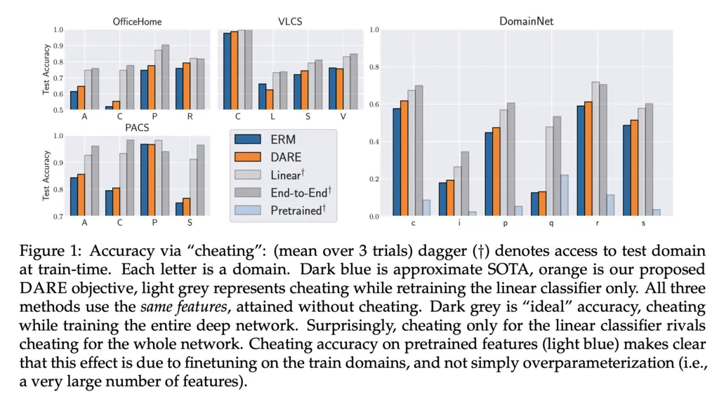
The paper investigates this by the following experiment.

Train a model on just the training dataset. Then freeze the features and allow it to “cheat” by fine-tuning a linear classifier on samples from the test domain (note that this is not the same as the test set).
Train another model on both the training data and allow full-parameter updates on the samples from the test domain.

The difference between the two setups is whether training on just points from the train domain allows the model to learn features that suffice for the test domain.

They found that performance in both cases was comparable, indicating that the features learnt using ERM are already good enough, and the main remaining bottleneck is in learning a good predictor that generalizes:

3. DARE Training Objective

They propose an alternative to the ERM training objective, which they call Domain-Adjusted Regression (DARE):

\[\min _\beta \sum_{e \in \mathcal{E}} \mathbb{E}_{p^e}\left[\ell\left(\beta^T \Sigma_e^{-1 / 2} x, y\right)\right] \quad \text{ subject to softmax }\left(\beta^T \Sigma_e^{-1 / 2} \mu_e\right)=\frac{1}{k} \mathbf{1} , \qquad \forall e \in \mathcal{E}\]

Let’s break it down:

\(\mathcal{E}\) represents the set of possible environments. In something like image classification, this could be things like the weather, climate, lighting, etc. In general, it is the different ways that things could vary that are not directly relevant to the task/which models may otherwise learn spurious correlations from.
\(\ell\) is the multinomial logistic loss
For an environment \(e\), \(p^e(x,y)\) gives the distribution over features \(x\) and class labels \(y\)
\(\Sigma_e\) is the covariance matrix of the feature in environment \(e\)
\(\beta\) is the matrix of transformation to be optimized for

In essence, it is saying:

we want to find some linear transformation \(\beta\) of the whitened (meaning changed to zero mean unit covariance) input features such that,
it does well on all environments (via a summation),
and doing well means minimizing the loss on the predictions between the whitened features transformed by \(\beta\) against \(y\),
and we also want to constrain it such that for any environment, the predictions of this transformation on the whitened features on the mean of the features give equal probability across all class labels.

We don’t need to subtract the mean from the whitening transformation, because the softmax loss is shift-invariant for its features.

The DARE objective is convex as both the objective function and feasible set defined by the constraints are convex, making it easy to optimize for by taking the Lagrangian.

Most Glaring Deficiency

Mostly a skill/background issue on my end, but the level of technicality of exposition between Sections 1-2 and Sections 3-5 increased dramatically, and it was quite difficult to follow without the right background.

Conclusions for Future Work

The work suggests that deep networks have already learned the right representations, and so in many cases fine-tuning on just a linear classifier could be sufficient to get very competitive performance compared to full-parameter fine-tuning.