LoRA: Low-Rank Adaptation of Large Language Models

An important paradigm of natural language processing consists of large-scale pre-training on general domain data and adaptation to particular tasks or domains. As we pre-train larger models, full fine-tuning, which retrains all model parameters, becomes less feasible. Using GPT-3 175B as an example – deploying independent instances of fine-tuned models, each with 175B parameters, is prohibitively expensive. We propose Low-Rank Adaptation, or LoRA, which freezes the pre-trained model weights and injects trainable rank decomposition matrices into each layer of the Transformer architecture, greatly reducing the number of trainable parameters for downstream tasks. Compared to GPT-3 175B fine-tuned with Adam, LoRA can reduce the number of trainable parameters by 10,000 times and the GPU memory requirement by 3 times. LoRA performs on-par or better than fine-tuning in model quality on RoBERTa, DeBERTa, GPT-2, and GPT-3, despite having fewer trainable parameters, a higher training throughput, and, unlike adapters, no additional inference latency. We also provide an empirical investigation into rank-deficiency in language model adaptation, which sheds light on the efficacy of LoRA. We release a package that facilitates the integration of LoRA with PyTorch models and provide our implementations and model checkpoints for RoBERTa, DeBERTa, and GPT-2 at https://github.com/microsoft/LoRA.

Three Important Things

1. LoRA

This paper introduces Low-Rank Adaptation (LoRA), which is a technique for efficient fine-tuning.

In normal fine-tuning, all the parameters of the model are updated. However, this is expensive and not practical for large models on consumer hardware.

On the other hand, in LoRA, the pre-trained parameters are frozen, and only a low-dimensional subset of the parameters are trainable.

For instance, in the case of a weight matrix (i.e the projection matrices for query/key/values/outputs in Transformers), if \(W_0 \in \R^{d \times k}\) represents the original weight matrix, then instead of learning a new fine-tuned \(W\) that requires all \(dk\) parameters to be updated, we can factorize this update \(W = W_0 + \Delta W\) with low-rank decomposition \(\Delta W = BA\), where \(B \in \R^{d \times r}, A \in \R^{r \times k}\), where \(r\) is significantly smaller than \(d\) and \(k\). In this way, we only have to update \(r(d+k)\) parameters instead.

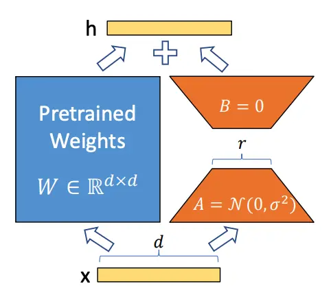
The diagram above illustrates how this works. \(A\) is initialized with random Gaussians, and \(B\) is initialized with zero. During the forward pass, the input \(x\) can be applied to both the pre-trained weights and the low-rank adaptation layer, and summed up:

\[h=W_0 x+\Delta W x=W_0 x+B A x\]

In the paper, they compare LoRA with existing techniques for efficient fine-tuning:

Adapter Layers: this introduces adding additional adapter layers that contain relatively few parameters and hence doesn’t add much in the way of overall computation. However, the downside is that these adapter layers still must be processed sequentially, which presents an additional latency cost for inference.
Prefix-tuning: Another approach is prefix tuning, where a special prefix is prepended to adapt it to the task at hand. However, optimizing for this prefix is hard, and it also reduces the remaining amount of tokens for the task.

2. LoRA Benefits

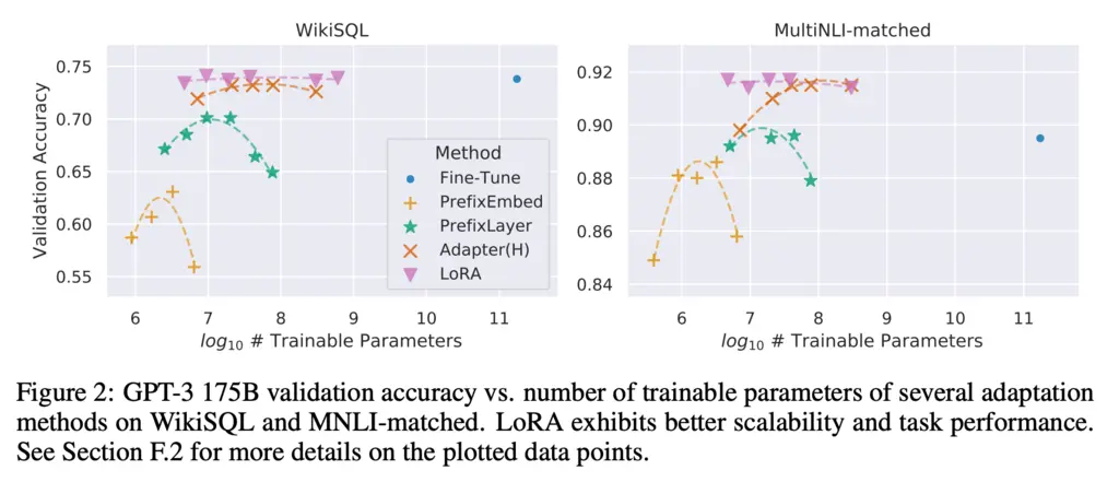
Empirically, even with very low rank, LoRA performs competitively against full-parameter fine-tuning and even surpasses it:

It’s possible to fine-tune many different light-weight adapters for different tasks using the same base model. During inference time, you can dynamically swap out for the appropriate \(A, B\) matrices for the task at hand while sharing the same base model, allowing you to serve many different models without having to incur the cost of needing to provision an equivalent number of full-parameter fine-tuned models.

In fact, there are startups like Predibase whose business model is doing precisely this for customers.

3. Why LoRA Works

The author’s original motivation for LoRA is that over-parameterized models have intrinsic low-rank structures after training, and so only a low-rank update is required to fine-tune a pre-trained model.

To do so, they analyzed the subspace similarity of the \(A_{r=8}\) and \(A_{r=64}\), which is the first adapter matrix that the input is projected onto of rank 8 and 64 respectively.

Given some matrix \(A\), you can perform the SVD decomposition \(A = U \Sigma V^T\), where both \(U, V\) are orthonormal matrices. To compare subspace similarity, they compared \(U_{A_{r=8}}\) and \(U_{A_{r=64}}\), which is in the span of \(A_{r=8}\) and \(A_{r=64}\) respectively, using Grassman distance:

\[\phi\left(A_{r=8}, A_{r=64}, i, j\right)=\frac{\left\|U_{A_{r=8}}^{i \top} U_{A_{r=64}}^j\right\|_F^2}{\min (i, j)} \in[0,1],\]

where \(U^i_{A_{r=8}}\) are the columns of \(U_{A_{r=8}}\) truncated to the top-\(i\) singular vectors, and similarly for \(U^i_{A_{r=64}}\).

To understand what the metric is doing, it is saying that when we consider only the top \(i\) and \(j\) singular vectors of \(U^i_{A_{r=8}}\) and \(U^i_{A_{r=64}}\) respectively, and take all the pairwise dot-product of their columns, which gives \(i * j\) dot products. However, the maximum sum that can be achieved is \(\min(i, j)\), since it is constrained by the rank of the smaller subspace, and hence we normalize by that factor.

Here are the results:

From the plots, we see that there is strong subspace similarity when just taking the top \(i\) singular values for \(U^i_{A_{r=8}}\) against \(U^i_{A_{r=64}}\) for any \(j\), and this begins to decay as \(i\) increases. In fact, when \(i=1\) the Grassman distance was over 0.5, which was corroborated by their empirical results that even rank 1 LoRA performed well.

This shows that a low-rank adapter is sufficient for LoRA to capture the direction of most of the interesting changes.

Most Glaring Deficiency

I am not sure why the weight matrices for the feedforward networks were not included in the components which the authors experimented with applying LoRA to. They considered the key, query, value matrices in self-attention, as well as the output projection matrices for multi-head attention. The feedforward networks seemed like another clear place to try.

Conclusions for Future Work

The more we understand the inner workings of a problem, the more we can exploit its idiosyncrasies to achieve some sort of relaxation that still respects the general properties of the problem. In this case, both empirical and theoretical understanding of the low-rank structure of updates gave birth to this highly-influential method used for fine-tuning LLMs and diffusion models today.