LongRoPE: Extending LLM Context Window Beyond 2 Million Tokens

Large context window is a desirable feature in large language models (LLMs). However, due to high fine-tuning costs, scarcity of long texts, and catastrophic values introduced by new token positions, current extended context windows are limited to around 128k tokens. This paper introduces LongRoPE that, for the first time, extends the context window of pre-trained LLMs to an impressive 2048k tokens, with up to only 1k fine-tuning steps at within 256k training lengths, while maintaining performance at the original short context window. This is achieved by three key innovations: (i) we identify and exploit two forms of non-uniformities in positional interpolation through an efficient search, providing a better initialization for fine-tuning and enabling an 8x extension in non-fine-tuning scenarios; (ii) we introduce a progressive extension strategy that first fine-tunes a 256k length LLM and then conducts a second positional interpolation on the fine-tuned extended LLM to achieve a 2048k context window; (iii) we readjust LongRoPE on 8k length to recover the short context window performance. Extensive experiments on LLaMA2 and Mistral across various tasks demonstrate the effectiveness of our method. Models extended via LongRoPE retain the original architecture with minor modifications to the positional embedding, and can reuse most pre-existing optimizations.

Three Important Things

1. Linear Positional Interpolation Is Suboptimal

To achieve long context length LLMs, one thing that must be addressed is getting positional embeddings that still work well at this large context length. This is challenging since long data that has such length is rare, and training on such long context windows is very expensive computationally.

The paper aims to answer the question of how we can train a LLM using a small context window (so it is more efficient), but then extend it to a much longer context during production. They analyze this from the direction of the positional embeddings that are used.

To do so, they build on RoPE. Recall that in RoPE, the token at position \(n\) has the following \(d\)-dimensional embedding, where \(\theta_i = \theta^{-2i/d}\) are the rotation frequencies:

\[\left[ \cos(n \theta_0), \sin(n \theta_0), \cos(n \theta_1), \cdots, \cos(n \theta_{d/2-1}), \sin(n \theta_{d/2-1}) \right].\]

The ratio between the new context length \(L'\) and the current context length \(L\) is the context window extension ratio: \(s = \frac{L'}{L}\). If we just naively extend RoPE to a longer context length by this ratio, then since now we have more positions, for the different positions to be unique, we’ll need to decrease our frequencies by a similar amount. Suppose we do this for rescale factor \(\lambda\), then we get:

\[\left[ \cos(n \theta_0/\lambda), \sin(n \theta_0/\lambda), \cos(n \theta_1/\lambda), \cdots, \cos(n \theta_{d/2-1}/\lambda), \sin(n \theta_{d/2-1}/\lambda) \right].\]

Decreasing this frequency linearly by dividing the frequencies by the context length extension ratio gives rise to a technique known as linear positional interpolation (PI), where we set \(\lambda = s\).

However, this does not perform well as it causes nearby indices to be indistinguishable from one another, since they now take on more similar values due to the lower frequency. This phenomenon is made worse as the extension ratio increases.

The paper also cited another NTK-based interpolation method that this tries to improve on, but it was hard to understand what this technique was doing and the motivation behind it as it was from a Reddit thread that was rather brief.

2. 2 Sources of Non-Uniformity for LongRoPE

The 2 changes that they propose are the following (which they call the 2 sources of non-uniformity):

Instead of having a fixed \(\lambda\) across all dimension indices, we can try to search for good values \(\lambda_i\) for each index \(i\). This was done via evolution search (why not make this a learnable parameter that can be found by gradient descent?). They used perplexity as a measure of fitness for the genetic algorithm.
Initial tokens should not be subject to interpolation, as starting tokens tend to be attended to by the attention mechanism, and hence interpolation could cause performance degradation, especially without fine-tuning. They denote the optimal number of starting tokens that do not undergo interpolation as \(\hat{n}\). All tokens after the \(\hat{n}\)th token will go through interpolation.

Visually, it looks like the following, where I believe there’s an error with the diagram on the third row for RoPE:

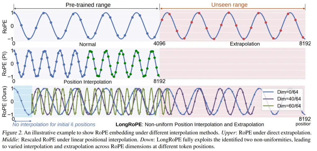
The first row shows what RoPE would do if we just extrapolated it to the new indices when extending the context window. This may cause it to perform poorly on the new indices that it has not seen before during training.

The second row shows what it would look like using the positional interpolation. Since the context window was doubled, we halve the frequency so that now what used to be at token 1 is now at token 2, what used to be at token 32 is now at token 64, and so on. The diagram looks somewhat misleading since the x-series scale was changed to be doubly compressed, but essentially we’re now still operating in the same regime of values as during training, except it is interpolated (which is an ok thing to do since neural networks are great at interpolating things).

The final row shows the LongRoPE technique. The shaded blue region on the left indicates the initial \(\hat{n}\) tokens that are not subject to any interpolation, and uses the original RoPE embeddings. After this regime, we see sample positional encoding values at different dimension indices for the different positions.

I believe that there’s an error in the figure, where the lower dimensions should have higher frequencies, and the higher dimensions with lower frequencies. This is because in practice they added the additional monotonic constraint \(\lambda_i \leq \lambda_{i+1}\) to reduce the search space of their evolutionary algorithm.

3. Building LongRoPE

The way they trained LongRoPE was quite interesting.

First, they took a base model (both LLaMA2-7B and Mistral-7B), and originally with context length 4k.
They then used LongRoPE search to increase to context window size 128k (32x) and 256k (64x).
They fine-tune on 256k context using rescaled parameters (which I believe means positional interpolation) for 128k for 400 steps. They then swapped this out for the 256k parameters and fine-tuned for another 600 steps. They claim that doing so is more efficient than directly fine-tuning to 256k, but I don’t really see why since the only difference is on the values for \(\lambda_i\) and \(\hat{n}\) that they used.
Finally, they extend again to 2048k with another round of LongRoPE search, to get a 2048k context-length model with extension ratio 512x.

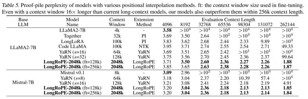
Here are some results, where it performs well on perplexity evals on the Proof-Pile even at very long context lengths, whereas both of the other baselines blow up:

Most Glaring Deficiency

The choice of an evolutionary search algorithm to find the right non-uniformity parameters felt slightly odd. What about other methods traditionally used in hyperparameter search like Bayesian optimization, or perhaps make the \(\lambda_i\) learnable parameters in itself, like learned positional embeddings?

Some parts of the design also felt quite hacky, like how they cased on whether the context was short enough in order to adjust the rescaling factors, in order to address issues with degraded performance at short context lengths. This hurts the generalizability of the approach if special cases must be considered.

Conclusions for Future Work

Similar ideas of realizing that we can use non-uniformity of parameters to get better performance, but doing so in a smart and computational efficient way can help derive gains in other areas of machine learning.