ColBERT: Efficient and Effective Passage Search via Contextualized Late Interaction over BERT

Recent progress in Natural Language Understanding (NLU) is driving fast-paced advances in Information Retrieval (IR), largely owed to fine-tuning deep language models (LMs) for document ranking. While remarkably effective, the ranking models based on these LMs increase computational cost by orders of magnitude over prior approaches, particularly as they must feed each query-document pair through a massive neural network to compute a single relevance score. To tackle this, we present ColBERT, a novel ranking model that adapts deep LMs (in particular, BERT) for efficient retrieval. ColBERT introduces a late interaction architecture that independently encodes the query and the document using BERT and then employs a cheap yet powerful interaction step that models their fine-grained similarity. By delaying and yet retaining this fine-granular interaction, ColBERT can leverage the expressiveness of deep LMs while simultaneously gaining the ability to pre-compute document representations offline, considerably speeding up query processing. Beyond reducing the cost of re-ranking the documents retrieved by a traditional model, ColBERT’s pruning-friendly interaction mechanism enables leveraging vector-similarity indexes for end-to-end retrieval directly from a large document collection. We extensively evaluate ColBERT using two recent passage search datasets. Results show that ColBERT’s effectiveness is competitive with existing BERT-based models (and outperforms every non-BERT baseline), while executing two orders-of-magnitude faster and requiring four orders-of-magnitude fewer FLOPs per query.

Three Important Things

1. Existing Neural Information Retrieval Techniques

Neural information retrieval techniques use neural networks instead of hand-crafted features (i.e BM25) to rank similarity between queries and documents. This paper introduces ColBERT, which improves on BERT-based retrieval techniques by being computationally more efficient.

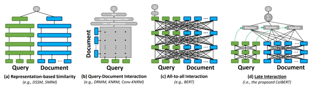
Let’s first survey the landscape of retrieval techniques, with respect to the figure above:

(a) Representation-based Similarity: this is probably the most well-known approach, where the document chunks are embedded offline through some deep neural network, and the query chunks are embedded similarly but online. Pairwise similarity scores are computed between the query against all documents, and the top ones are returned.
(b) Query-Document Interaction: in this approach, word and phrase-level relationships (using n-grams) are computed between all words in the query and documents as a form of feature engineering, and these relationships are converted into an interaction matrix that is fed as input to a deep neural network.
(c) All-to-all Interaction: This can be viewed as a generalization of (b), where all pairwise interactions both within and across the query and document are considered. This is achieved via self-attention, with BERT being used in practice since it is bi-directional and hence can actually model all pairwise interactions, instead of just causal relationships.
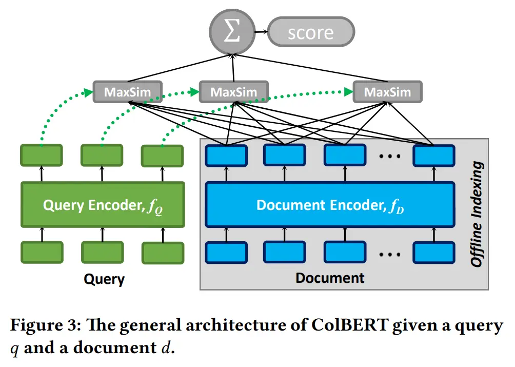
(d) Late Interaction: this is the approach introduced by the paper, where the document embeddings can be computed offline with BERT, and then compute the query embeddings online. They then take what they call the MaxSim operator (explained later) between the embeddings from the query and document. This architecture is visualized below:

2. ColBERT Query and Document Encoder

Let’s understand how query encoder and document encoder works in detail. Below, \(E_q, E_d\) provide the setup for getting the output embeddings from the query encoder and document encoder respectively.

\[\begin{aligned} & \left.\left.E_q:=\text { Normalize( CNN( BERT([Q] } q_0 q_1 \ldots q_l \# \# \ldots \# \# \right)\right)) \\ & \left.\left.\left.E_d:=\text { Filter( Normalize( CNN( BERT([D] }d_0 d_1 \ldots d_n \right)\right)\right)\end{aligned}\]

To distinguish between the query and documents when they are passed as input into BERT, the authors prepend a special token [Q] and [D] before queries and documents respectively. Mask tokens are used to pad inputs up to the context window length, denoted by \(\#\) above. Why did they not add mask tokens for the document? I’m not sure, but my guess is that documents are usually context-window limited and hence are already truncated and require no further padding.

Next, in both cases we pass the inputs to BERT, before applying them to a fully connected layer (without an activation). I’m not sure why they denoted this by \(\textrm{CNN}\) instead of something like \(\textrm{MLP}\), it could be the case that they are viewing the different embeddings as coming from different channels and hence see this as a form of convolution.

Finally, the \(\textrm{Normalize}\) step rescales the embedding such that it has L2 norm of one, and \(\textrm{Filter}\) (which is only applicable for the document encoders) strips embeddings corresponding to punctuation symbols, as the authors believe they are unnecessary for the performance of the IR system and only add computational overhead.

3. ColBERT Relevancy Scores

With all the embedding steps behind us, how do we compute a score between a query \(q\) and document \(d\)? To do this, the authors used the following formulation of relevancy scores \(S_{q,d}\):

\[S_{q, d}:=\sum_{i \in\left[\left|E_q\right|\right]} \max _{j \in\left[\left|E_d\right|\right]} E_{q_i} \cdot E_{d_j}^T\]

This is saying that the score between \(q\) and \(d\) is computed by first going through the embeddings of every single token in the query, and then finding the embedding in the document that maximizes their dot product, which is a measure of how similar the two embeddings are.

Their formulation is somewhat reminiscent of Gaussian complexity, where we try to understand how expressive a function class \(K\) is based on how well it can fit random noise:

\[\mathcal{G}(K)=\mathbb{E}_{\epsilon \sim \mathcal{N}\left(0, I_d \right)}\left[\sup _{\theta \in K}\langle\epsilon, \theta\rangle\right]\]

Finally, to train ColBERT, they used triples \(\langle q, d^+, d^- \rangle\) containing the query \(q\), a positive document \(d^+\) and negative document \(d^-\) to minimize the softmax cross-entropy loss.

Most Glaring Deficiency

At the end of the day, I did not really find this paper very novel, as their main technical contribution is just how they computed the relevancy scores when viewed from the lens of the representation-based similarity approach (as this already makes use of late interaction).

Indeed, this technique could have also been extended to work with representation-based similarity, and so I feel like they missed a chance to solve a more general problem which seemed quite obvious.

However, I’ll admit I may have been unable to fully appreciate the merits of this paper, as I’m not very well-versed in the information retrieval literature.

Conclusions for Future Work

The technique of late interaction can be used to optimize systems, since it offers opportunities for offline pre-computation, and also may require less data to be processed at once (which can be an issue for superlinear-scaling algorithms like Transformers), at the cost of potentially slightly worse performance.