Matryoshka Representation Learning

Learned representations are a central component in modern ML systems, serving a multitude of downstream tasks. When training such representations, it is often the case that computational and statistical constraints for each downstream task are unknown. In this context rigid, fixed capacity representations can be either over or under-accommodating to the task at hand. This leads us to ask: can we design a flexible representation that can adapt to multiple downstream tasks with varying computational resources? Our main contribution is Matryoshka Representation Learning (MRL) which encodes information at different granularities and allows a single embedding to adapt to the computational constraints of downstream tasks. MRL minimally modifies existing representation learning pipelines and imposes no additional cost during inference and deployment. MRL learns coarse-to-fine representations that are at least as accurate and rich as independently trained low-dimensional representations. The flexibility within the learned Matryoshka Representations offer: (a) up to 14x smaller embedding size for ImageNet-1K classification at the same level of accuracy; (b) up to 14x real-world speed-ups for large-scale retrieval on ImageNet-1K and 4K; and (c) up to 2% accuracy improvements for long-tail few-shot classification, all while being as robust as the original representations. Finally, we show that MRL extends seamlessly to web-scale datasets (ImageNet, JFT) across various modalities – vision (ViT, ResNet), vision + language (ALIGN) and language (BERT). MRL code and pretrained models are open-sourced at https://github.com/RAIVNLab/MRL.

Three Important Things

1. The Problem with Fixed Feature (FF) Representations

Learned representations are essential for extracting useful features from data, making downstream tasks significantly easier. Such representations have a fixed size, and need to have a large number of dimensions in order to be sufficiently expressive for any task.

However, such high-dimensional representations impose a computational overhead on tasks that may not require such a high degree of fidelity, which motivates the need for a flexible representation architecture that can perform feature mappings across a range of dimensions, at the potential cost of a loss of accuracy on downstream tasks.

2. Matryoshka Representation Learning (MRL)

To do so, the authors introduce Matryoshka Representation Learning (MRL), a technique that provides representations at \(O(\log (d))\) chosen representation sizes, where \(d\) is the highest-dimension representation we care about. The name is chosen due to how it is reminiscent of the nested Russian Matryoshka dolls.

We will first describe how MRL is trained, and in the next section explain how it can utilized for adaptive retrieval and adaptive classification tasks that run much faster than fixed feature representations.

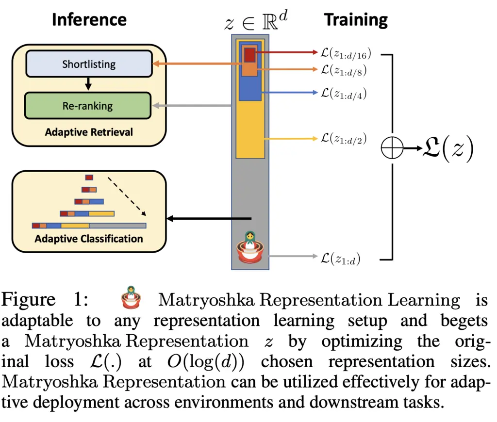
Unsurprisingly, the representation \(z\) is trained by a deep neural network parameterized by \(\theta_F\), given by \(F (\, \cdot \,; \theta_F) : \chi \to \R^d\). We consider a set \(\calM\) of representation sizes, where \(| \calM | \leq \lfloor \log(d) \rfloor\). For instance, in the paper \(\calM = \left\{ 8, 16, \dots, 1024, 2048 \right\}\).

In the paper, MRL is trained on a multi-class classification problem, though the same idea can be adapted to other domains. Then we have a dataset of \(N\) input-label pairs \(x_i, y_i\). To solve this multi-class classification problem, for each representation size \(m \in \calM\), they apply a single trained linear layer \(\bW^{(m)}\) to the representation and then take the multi-class softmax cross-entropy loss function \(\calL\).

This gives the following loss formulation:

\[\begin{align*} \min _{\left\{\mathbf{W}^{(m)}\right\}_{m \in \mathcal{M}}, \theta_F} \frac{1}{N} \sum_{i \in[N]} \sum_{m \in \mathcal{M}} c_m \cdot \mathcal{L}\left(\mathbf{W}^{(m)} \cdot F\left(x_i ; \theta_F\right)_{1: m} ; y_i\right) \end{align*},\]

where we jointly optimize over the projection weights for each representation level and the parameters for \(F\), and also allow for a scaling factor \(c_m\) to weigh the importance of each representation level. Note too that we only take the first \(m\) dimensions from \(F\) for each \(m\).

To reduce the number of parameters, one can perform weight tying between the \(\bW^{m}\) where they overlap, which roughly halves the number of parameters.

As such, the trained MRL \(F\) is encouraged to learn a representation that works well for some representative downstream task over all representation levels, that hopefully also generalizes.

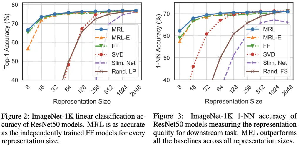
The following results show that MRL outperforms even fixed feature models, which is a very strong baseline. MRL-E denotes MRL with weight tying, which predictably performs slightly worse. SVD refers to dimensionality reduction using SVD, slim net are slimmable networks, and Rand. FS are randomly selected features from the highest capacity FF model.

3. Adaptive Classification and Adaptive Retrieval

We consider two main applications of MRL that can significantly speed things up.

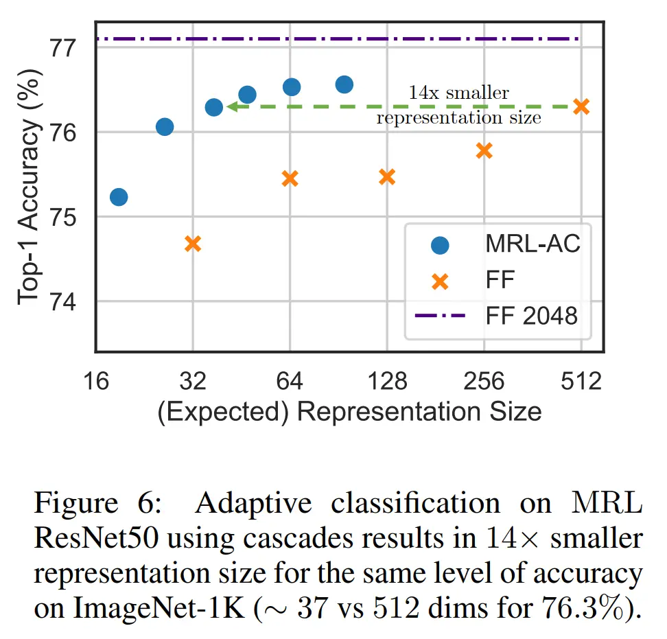
The first is adaptive classification, where we try to start with performing classification with a coarser representation, before moving on to a finer representation if we are not confident of its predictions.

Determining this confidence is done by previously learning some thresholds for these softmax probabilities on a holdout validation set, and then upgrading to a higher-capacity representation if it falls below this threshold.

Impressively, MRL was able to get the same accuracy as fixed feature baselines while using a 14x smaller representation:
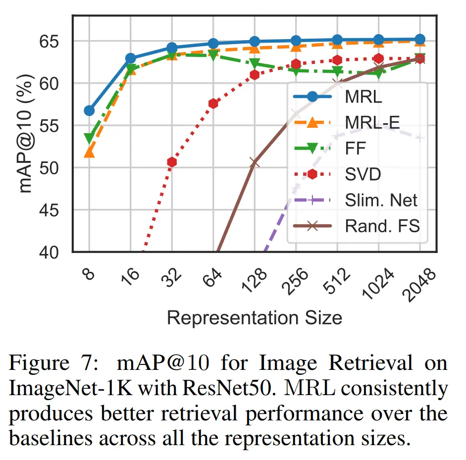
The other is adaptive retrieval, where we first retrieve a larger quantity of vectors using a lower-dimensional representation, before re-ranking the top ones using a higher dimension, hence saving on compute.

To compare retrieval against the other baselines, they used the mean Average Precision @ k (mAP@k) metric, where the top 10 closest embeddings are retrieved, and the mean of the number of embeddings whose label matches the label of the query label is taken.

Most Glaring Deficiency

Given the recent surge of interest in LLMs, the paper could have also done some experiments with language modeling tasks. Language modeling can be viewed as a form of sequential multi-class classification problem, so it seems like quite a natural direction to pursue.

Conclusions for Future Work

Instead of using fixed-size representations, we can utilize flexible representation learning approaches that encodes information at multiple granularities in a single embedding vector.

Perhaps we can use similar ideas to also get flexibility at other kinds of computational and memory bottlenecks, where we may not require the full ambient dimension to perform well for the task at hand.