High-Resolution Image Synthesis with Latent Diffusion Models

By decomposing the image formation process into a sequential application of denoising autoencoders, diffusion models (DMs) achieve state-of-the-art synthesis results on image data and beyond. Additionally, their formulation allows for a guiding mechanism to control the image generation process without retraining. However, since these models typically operate directly in pixel space, optimization of powerful DMs often consumes hundreds of GPU days and inference is expensive due to sequential evaluations. To enable DM training on limited computational resources while retaining their quality and flexibility, we apply them in the latent space of powerful pretrained autoencoders. In contrast to previous work, training diffusion models on such a representation allows for the first time to reach a near-optimal point between complexity reduction and detail preservation, greatly boosting visual fidelity. By introducing cross-attention layers into the model architecture, we turn diffusion models into powerful and flexible generators for general conditioning inputs such as text or bounding boxes and high-resolution synthesis becomes possible in a convolutional manner. Our latent diffusion models (LDMs) achieve a new state of the art for image inpainting and highly competitive performance on various tasks, including unconditional image generation, semantic scene synthesis, and super-resolution, while significantly reducing computational requirements compared to pixel-based DMs. Code is available at https://github.com/CompVis/latent-diffusion .

Three Important Things

1. Diffusion Models in Latent Space

The problem with diffusion models is that in spite of their recent impressive results that is on-par with GANs, they are very computationally demanding to train, where it takes hundreds of GPU days to train a powerful state-of-the-art diffusion model. This is because the maximum-likelihood objective in diffusion models causes it to spend a disproportionate amount of time modeling small imperceptible details in pixel space that are imperceptible.

The authors instead propose to train the diffusion models in latent space, where the encoder performs perceptual compression by stripping away high-frequency information that is largely imperceptible, allowing us to still model high-quality images while operating in a much lower-dimensional space.

Some of their results:

The original objective of diffusion models can be simplified from its ELBO into

\[L_{D M}=\mathbb{E}_{x, \epsilon \sim \mathcal{N}(0,1), t}\left[\left\|\epsilon-\epsilon_\theta\left(x_t, t\right)\right\|_2^2\right],\]

where \(\epsilon_\theta\left(x_t, t\right)\) is the denoising autoencoder that predicts the noise for \(x_t\) conditioned on time step \(t\), and \(t\) is the time step. Therefore a smaller loss means it is better at predicting the added noise.

In latent diffusion models, we now operate with the latent \(z_t\) which comes from the encoder \(\mathcal{E}\), giving the objective

\[L_{L D M}:=\mathbb{E}_{\mathcal{E}(x), \epsilon \sim \mathcal{N}(0,1), t}\left[\left\|\epsilon-\epsilon_\theta\left(z_t, t\right)\right\|_2^2\right].\]

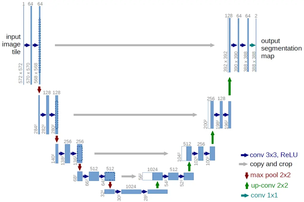
In practice, \(\epsilon_\theta\left(z_t, t\right)\) is a time-conditional ablated U-Net, which has good inductive bias towards image data. The U-Net architecture consists of downsampling layers via max pooling operations on one end, and upsampling layers on the other end, with intermediate layers connected by skip connections:

2. Conditioning with Attention

It would be desirable to have some control over the outputs of diffusion process by conditioning the process on other inputs like text, semantic maps, or other images for image-to-image translation tasks.

To do this, they incorporate the cross-attention mechanism into the U-Net so that the image synthesis process pays attention to the conditioned inputs. The conditioned inputs \(y\) are passed through an appropriate domain-specific encoder (such as Transformers for text input) \(\tau_\theta\). The attention mechanism is the same as that used originally in the Transformers paper:

\[\textrm{Attention} (Q, K, V)=\operatorname{softmax}\left(\frac{Q K^I}{\sqrt{d}}\right) \cdot V,\]

with the query, key and values defined as follows:

\(Q=W_Q^{(i)} \cdot \varphi_i\left(z_t\right)\),
\(K=W_K^{(i)} \cdot \tau_\theta(y)\),
\(V=W_V^{(i)} \cdot \tau_\theta(y)\),

where the weight matrices are learnable projection matrices and \(\varphi_i(z_t)\) is the flattened output of the U-Net \(\epsilon_\theta\).

The input-conditioned objective is then

\[L_{L D M}:=\mathbb{E}_{\mathcal{E}(x), y, \epsilon \sim \mathcal{N}(0,1), t}\left[\left\|\epsilon-\epsilon_\theta\left(z_t, t, \tau_\theta(y)\right)\right\|_2^2\right],\]

where we optimize over both the denoising network \(\epsilon_\theta\) as well as the input encoder \(\tau_\theta\).

3. Applications of Latent Diffusion Models

The paper explores various applications of their approach:

Text-to-image generation by conditioning on text, where they use a BERT-tokenizer and use a transformer to encode the inputs
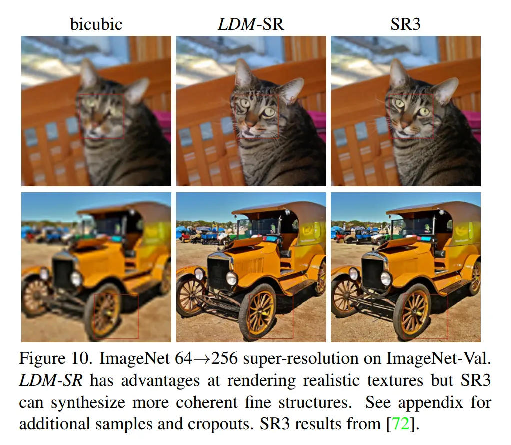
Image super-resolution. This is done by conditioning on concatenated inputs of the low-resolution input image.
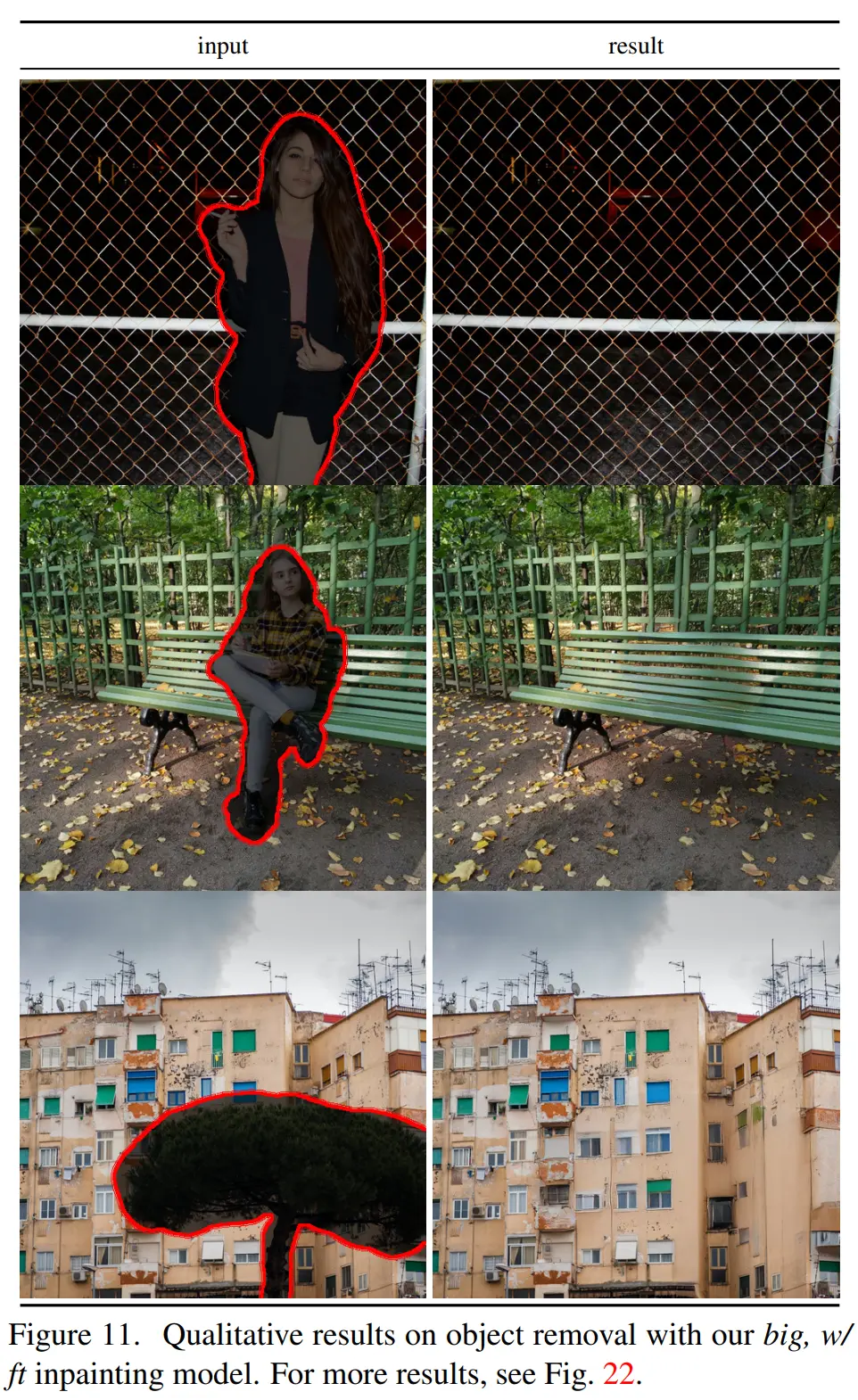
Image inpainting. This was also done by concatenating spatially-aligned inputs of the image to inpaint.

Most Glaring Deficiency

The cross-attention mechanism is key to how they performed conditional image synthesis, but there was not much ablation study done on how modifying this mechanism affected the results of the images generated. It is also not easy to train the huge attention matrix weights, especially more so now that we have an expensive image synthesis procedure, and so more details on how they managed to do so efficiently would have been useful.

Conclusions for Future Work

This paper was the foundation for Stable Diffusion, whose significance and popularity in the image generative AI space cannot be understated. A lot of subsequent research has built on this open-sourced model, and I think the legacy of this paper hence speaks for itself.

The idea of operating in latent space is not new, but helped to democratize access to diffusion models for the vast majority of GPU-poor researchers and hobbyists. Similar ideas could be applied when we face computational bottlenecks operating in sample space.