The Implicit Bias of Gradient Descent on Separable Data

We examine gradient descent on unregularized logistic regression problems, with homogeneous linear predictors on linearly separable datasets. We show the predictor converges to the direction of the max-margin (hard margin SVM) solution. The result also generalizes to other monotone decreasing loss functions with an infimum at infinity, to multi-class problems, and to training a weight layer in a deep network in a certain restricted setting. Furthermore, we show this convergence is very slow, and only logarithmic in the convergence of the loss itself. This can help explain the benefit of continuing to optimize the logistic or cross-entropy loss even after the training error is zero and the training loss is extremely small, and, as we show, even if the validation loss increases. Our methodology can also aid in understanding implicit regularization n more complex models and with other optimization methods.

Three Important Things

1. Gradient Descent On Separable Data Has Implicit Bias Towards Max-Margin SVM

Why is it that over-parameterized models fitted on training data via gradient descent actually generalizes well instead of overfitting? In this work, the authors make headway towards answering this question by showing that the solution found by gradient descent on linearly separable data actually has an implicit bias towards the \(L_2\) max-margin SVM solution, meaning that it will eventually converge to that solution (even as validation loss may be increasing).

As a brief recap of max-margin (also known as hard) SVM, consider the linearly separable dataset given in the figure below:

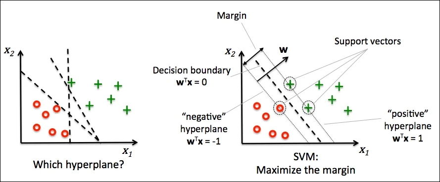
Max-margin SVM solution. Taken from Packt.

While there are infinitely many solutions of lines that result in perfect accuracy, the solution that maximizes the margin to the support vectors (i.e closest datapoints to the solution hyperplane on both sides of the plane) will be the one that generalizes the best.

Let’s now consider the problem setup: the goal is to minimize the empirical loss

\[\mathcal{L}(\bw) = \sum_{n=1}^N \ell \left( y_n \bw^\top \bx_n \right),\]

where labels \(y_n\) are binary \(\pm 1\) labels.

They make three key assumptions for their result:

Assumption 1: The dataset is linearly separable: \(\exists \bw_*\) such that \(\forall n : \bw_* \bx_n > 0\)

Assumption 2: The loss function \(\ell(u)\) is positive, differentiable, monotonically decreasing to zero, is a \(\beta\)-smooth function (derivative is \(\beta\)-Lipschitz), and \(\limsup_{u \to -\infty} \ell'(u) < 0\)

Assumption 3: The negative loss derivative \(-\ell'(u)\) has a tight exponential tail (i.e it decays exactly exponentially fast beyond some initial regime)

Using these assumptions, they showed the following result:

Theorem (Implicit Bias of Gradient Descent Towards Max-Margin SVM Solution)

For any dataset which is linearly separable (Assumption 1), any \( \beta \)-smooth decreasing loss function (Assumption 2) with an exponential tail (Assumption 3), any stepsize \( \eta<2 \beta^{-1} \sigma_{\max }^{-2}(\mathbf{X}) \) and any starting point \( \mathrm{w}(0) \), the gradient descent iterates \( \mathbf{w}(t) \) will behave as: \[ \mathbf{w}(t)=\hat{\mathbf{w}} \log t+\boldsymbol{\rho}(t), \] where \( \hat{\mathbf{w}} \) is the \( L_2 \) max margin vector (the solution to the hard margin SVM): \[ \hat{\mathbf{w}}=\underset{\mathbf{w} \in \mathbb{R}^d}{\operatorname{argmin}}\|\mathbf{w}\|^2 \text { s.t. } \mathbf{w}^{\top} \mathbf{x}_n \geq 1, \] and the residual grows at most as \( \|\rho(t)\|=O(\log \log (t)) \), and so \[ \lim _{t \rightarrow \infty} \frac{\mathbf{w}(t)}{\|\mathbf{w}(t)\|}=\frac{\hat{\mathbf{w}}}{\|\hat{\mathbf{w}}\|} \text {. } \] Furthermore, for almost all data sets (all except measure zero), the residual \( \rho(t) \) is bounded.

Let’s analyze what the theorem says.

First, we see that as the number of time steps increases, the magnitude of the weights \(\bw(t)\) will tend towards infinity, and it will be dominated by the \(\hat{\bw} \log t\) term, which grows much faster than \(\rho(t)\) which grows extremely slowly as \(O(\log \log (t))\).

Then this shows that the normalized weight vector tends towards \(\frac{\hat{\mathbf{w}}}{\|\hat{\mathbf{w}}\|}\), which is exactly the max-margin SVM solution.

However, one thing to note is that the rate of convergence to the max-margin solution is exponentially slow - since the growth of the weights is dominated by the \(\log t\) term, it will only converge in \(O\left( \frac{1}{\log t} \right)\).

This means that it is worthwhile to continue running gradient descent for a long time even when the loss is vanishingly small with zero training error.

2. Proof Sketch of Main Theorem

Why should this theorem be true? In this section, we’ll go through a quick sketch of the proof.

Assume for simplicity that the loss function is simply the exponential function \(\ell(u) = e^{-u}\).

First, they used previous results that gradient descent on a smooth loss function with an appropriate stepsize always converges. In other words, the gradient update eventually goes to 0. The gradient of the loss function is

\(\begin{align} -\nabla \mathcal{L}(\mathbf{w}) & = -\nabla \sum_{n=1}^N \ell \left( y_n \bw^\top \bx_n \right) \\ & = -\nabla \sum_{n=1}^N \exp \left( - y_n \bw^\top \bx_n \right) \\ & = \sum_{n=1}^N \exp \left(-\mathbf{w}(t)^{\top} \mathbf{x}_n\right) \mathbf{x}_n, \\ \end{align}\) and hence for this to go to zero, we require that \(-\bw(t)^\top \bx_n\) be driven to infinity, which means that the magnitude of \(\bw(t)\) will also go to infinity as only our weights change.

If we assume that \(\bw(t)\) converges to some limit \(\bw_{\infty}\) (this can be proven but we won’t do it here), then we can decompose it as

\[\bw(t) = g(t) \bw_{\infty} + \rho(t)\]

for some function \(g(t)\) that captures growth along \(\bw_{\infty}\), and residue term \(\rho(t)\).

Then we can re-write our gradient as \(\begin{align} -\nabla \mathcal{L}(\mathbf{w}) & =\sum_{n=1}^N \exp \left(-g(t) \mathbf{w}_{\infty}^{\top} \mathbf{x}_n\right) \exp \left(-\rho(t)^{\top} \mathbf{x}_n\right) \mathbf{x}_n. \end{align}\)

But as we increase \(t\) and \(g(t)\) correspondingly increases, then among all our \(n\) datapoints \(\bx_1, \cdots, \bx_n\), only those with the smallest values of \(\bw_{\infty}^\top \bx_n\) will meaningfully contribute to the gradient, and the contributions of the other terms with much larger values are negligible since we are taking the negative of these values in the exponent.

But then this means that the gradient update is effectively only dominated by contributions from some of these points - essentially the support vectors of the problem, like in SVM.

Then as we continue performing gradient updates such that \(\| \bw(t) \| \to \infty\), it is now essentially a linear combination of the support vectors.

This coincides with the KKT conditions for SVM:

\[\begin{align} & \hat{\bw} = \sum_{n=1}^N \alpha_n \bx_n \\ \text{such that} \qquad & \forall n\left(\alpha_n \geq 0 \text { and } \hat{\mathbf{w}}^{\top} \mathbf{x}_n=1\right) \text{ OR }\left(\alpha_n=0 \text { and } \hat{\mathbf{w}}^{\top} \mathbf{x}_n>1\right) \end{align}\]

and hence allows us to conclude that indeed \(\frac{\mathbf{w}}{\|\mathbf{w}\|}\) converges to \(\hat{\bw}\).

3. Empirical Evidence on Non-Separable Data

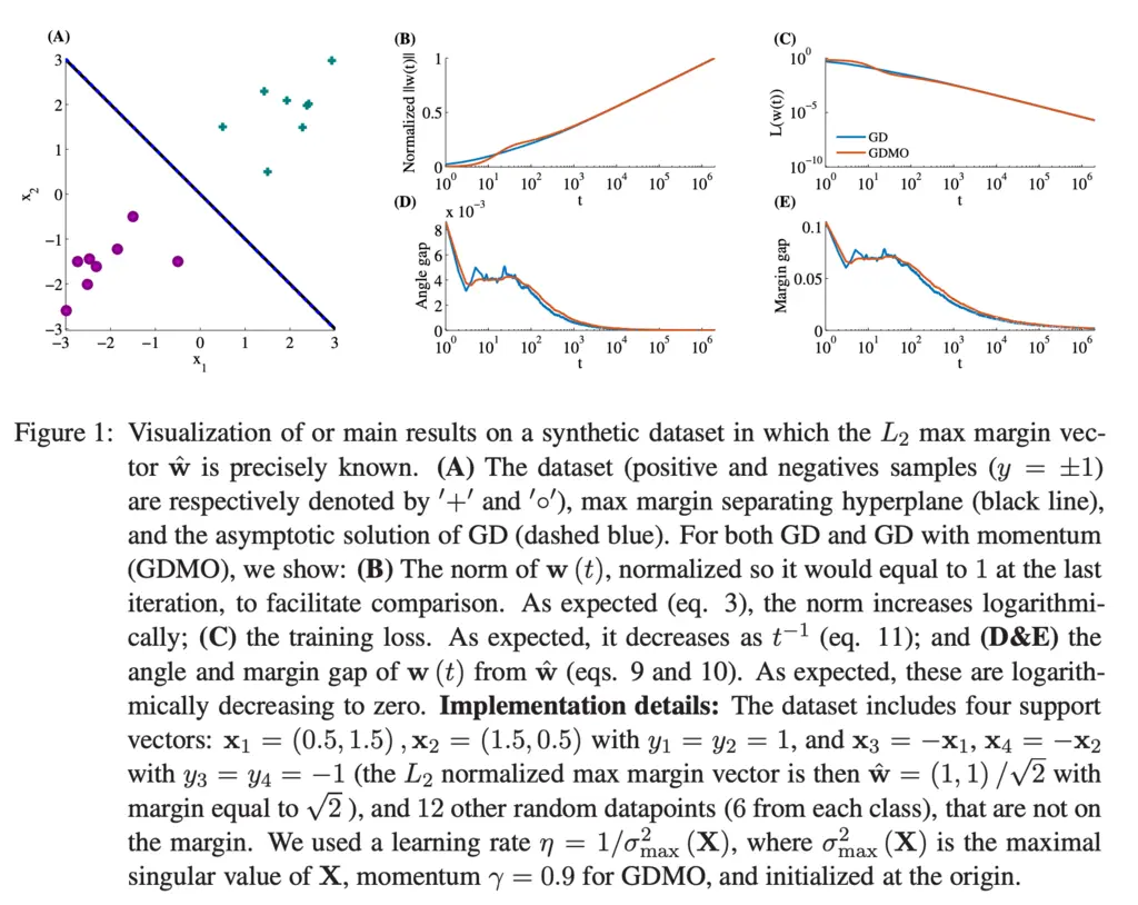
The authors showed that empirical results on synthetic data supported their theoretical findings:

A key objection to the generalizability of the main theorem is the extremely strong assumption that the data must be linearly separable.

The authors of course saw that coming, and also investigated the loss and error curves on non-linearly separable CIFAR10 dataset, and saw that it observed the same trends:

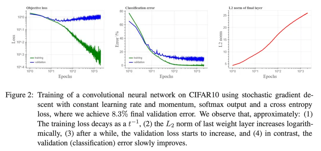
This is exciting, as it provides evidence that it may be possible to extend this theory to deep neural networks as well.

Most Glaring Deficiency

The result assumes the existence of some \(\bw_*\) that is capable of linearly separating the data, which is used in the proof that the weight iterates will have its magnitude eventually tend towards infinity, i.e \(\| \bw(t) \| \to \infty\).

It would be great if it is possible to show this without relying on this strong assumption as it is quite unrealistic as most real-world datasets are not linearly separable.

Conclusions for Future Work

Even when the training loss is zero or plateaus, it can be worthwhile to continue training. We should also look at the 0-1 error on the validation set instead of the validation loss, as it is possible that even though the validation loss increases, the 0-1 error actually improves and the model learns to generalize better.

As mentioned previously, it would be very exciting if the linearly separable assumption on the data can be theoretically removed, and if it can be extended to deeper neural networks.