Loss Landscapes and Optimization in Over-Parameterized Non-Linear Systems and Neural Networks

The success of deep learning is due, to a large extent, to the remarkable effectiveness of gradient-based optimization methods applied to large neural networks. The purpose of this work is to propose a modern view and a general mathematical framework for loss landscapes and efficient optimization in over-parameterized machine learning models and systems of non-linear equations, a setting that includes over-parameterized deep neural networks. Our starting observation is that optimization problems corresponding to such systems are generally not convex, even locally. We argue that instead they satisfy PL*, a variant of the Polyak-Lojasiewicz condition on most (but not all) of the parameter space, which guarantees both the existence of solutions and efficient optimization by (stochastic) gradient descent (SGD/GD). The PL* condition of these systems is closely related to the condition number of the tangent kernel associated to a non-linear system showing how a PL*-based non-linear theory parallels classical analyses of over-parameterized linear equations. We show that wide neural networks satisfy the PL* condition, which explains the (S)GD convergence to a global minimum. Finally we propose a relaxation of the PL* condition applicable to "almost" over-parameterized systems.

Three Important Things

1. Differences of Loss Landscape in Under-Parameterized and Over-Parameterized Models

Under-parameterized models are those where the number of parameters available is less than the number of (independent) constraints imposed on the network, and therefore it is unable to achieve 0 loss, defined as the mean-squared error on the given training data.

On the other hand, over-parameterized models have more parameters than constraints, and can therefore achieve 0 training loss.

Empirically, it has been observed that even though the optimization problem in over-parameterized models is highly non-convex, it still almost always manage to reach a global minimum, which is not the case for under-parameterized models. The huge success of large over-parameterized models has been a puzzling problem for many years.

This paper aims to answer why this is the case, and shows that the classic approach of viewing this problem from the lens of convexity is totally wrong and does not provide us with the machinery to answer this question:

“Convexity is not the right framework for analysis of over-parameterized systems, even locally.”

Instead, they introduce the PL$^*$ condition which is a variant of the Polyak-Łojasiewicz condition, and show that networks that satisfy the PL$^*$ condition can converge to a global minimum.

First, let’s look at the fundamental differences in the loss landscape of under-parameterized versus over-parameterized models:

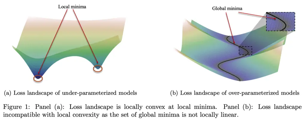
In under-parameterized models, there are many local minima which are locally convex. Local convexity means it is convex within some $\epsilon$-neighborhood of the local minima. This means that once we are sufficiently close to the local minimizer, then all our standard tools from convex optimization apply and we can see why gradient-based methods will minimize the loss.

However, in over-parameterized models, the loss landscape is in general not locally convex for any neighborhood around any minimizer. This is because there is non-zero curvature along the global minimas as illustrated in the figure above, resulting in a solution set that is non-convex. Since results from convexity theory requires both convex sets and functions, this shows that we cannot use it for analyzing the success of over-parameterized models.

2. PL$^*$ Condition for Analyzing Over-Parameterized Systems

We say that any function $f$ with $L$-Lipschitz first derivatives satisfies the Polyak-Łojasiewicz (PL) condition if for some $\mu > 0$, we have

\[\left\| \nabla f(w) \right\|^2 \geq \mu (f(w) - f^*), \qquad \forall w,\]

where $f^* = \argmin_{w \in \R^d} f(w)$ is the minimizer.

Polyak showed in 1963 that functions that satisfy the PL condition converge exponentially fast under gradient descent.

The authors introduce a modified variant called the PL$^*$ condition, with the main difference being our assumption that over-parameterized models can achieve 0 training loss and hence $f^*=0$, and that we only require the condition to hold in some subset $\mathcal{S}$ in the parameter space. Using a more suggestive $\mathcal{L}$ notation to denote the loss, this gives:

\[\left\| \nabla \mathcal{L}(w) \right\|^2 \geq \mu \mathcal{L}(w), \qquad \forall w \in \mathcal{S}.\]

The main result of the paper shows that satisfying the PL$^*$ condition in a ball guarantees the existence of solutions and fast convergence of both gradient descent and stochastic gradient descent, reproduced below (feel free to skip it):

Theorem (Local PL$^*$ condition implies existence of a solution + fast convergence)

Suppose the system $ \mathcal{F} $ is $ L_{\mathcal{F}} $-Lipschitz continuous and $ \beta_{\mathcal{F}} $-smooth. If the square loss $ \mathcal{L}(\mathbf{w}) $ satisfies the $ \mu $-PL $ L^* $ condition in the ball $ B\left(\mathbf{w}_0, R\right):=\left\{\mathbf{w} \in \mathbb{R}^m:\left\|\mathbf{w}-\mathbf{w}_0\right\| \leq R\right\} $ with $ R=\frac{2 L_{\mathcal{F}}\left\|\mathcal{F}\left(\mathbf{w}_0\right)-\mathbf{y}\right\|}{\mu} $. Then we have the following:

Existence of a solution: There exists a solution (global minimizer of $ \mathcal{L} $ ) $ \mathbf{w}^* \in B\left(\mathbf{w}_0, R\right) $, such that $ \mathcal{F}\left(\mathbf{w}^*\right)=\mathbf{y} $.
Convergence of GD: Gradient descent with a step size $ \eta \leq 1 /\left(L_{\mathcal{F}}^2+\beta_{\mathcal{F}}\left\|\mathcal{F}\left(\mathbf{w}_0\right)-\mathbf{y}\right\|\right) $ converges to a global solution in $ B\left(\mathbf{w}_0, R\right) $, with an exponential (a.k.a. linear) convergence rate: $$ \mathcal{L}\left(\mathbf{w}_t\right) \leq\left(1-\kappa_{\mathcal{F}}^{-1}\left(B\left(\mathbf{w}_0, R\right)\right)\right)^t \mathcal{L}\left(\mathbf{w}_0\right) . $$ where the condition number $\kappa_{\mathcal{F}}\left(B\left(\mathbf{w}_0, R\right)\right)=\frac{1}{\eta \mu}$.

This theorem was also extended to stochastic gradient descent in the paper.

3. Satisfying the PL$^*$ Condition

From the main theorem, systems that satisfy the PL$^*$ condition have nice properties like the existence of a globally minimal solution, and fast convergence to this solution. However, when does this condition hold?

The authors showed that wide neural networks satisfy the PL$^*$ condition. In this paper, neural networks are the standard stacked layers with fully connected layers and a bias term, and a twice-differentiable activation function, with $m$ defined as the minimum width of neurons on any layer. Then neural networks with sufficiently large $m$ will satisfy the PL$^*$ condition, made precise with their result:

Theorem (Wide neural networks satisfy PL* condition)

Consider the neural network $ f(\mathbf{W} ; \mathbf{x}) $, and a random parameter setting $ \mathbf{W}_0 $ such that $ W_0^{(l)} \sim \mathcal{N}\left(0, I_{m_l \times m_{l-1}}\right) $ for $ l \in[L+1] $. Suppose that the last layer activation $ \sigma_{L+1} $ satisfies $ \left|\sigma_{L+1}^{\prime}(z)\right| \geq \rho>0 $ and that $ \lambda_0:=\lambda_{\min }\left(K\left(\mathbf{W}_0\right)\right)>0 $. For any $ \mu \in\left(0, \lambda_0 \rho^2\right) $, if the width of the network $$ m=\tilde{\Omega}\left(\frac{n R^{6 L+2}}{\left(\lambda_0-\mu \rho^{-2}\right)^2}\right), $$ then $ \mu-P L^* $ condition holds the square loss function in the ball $ B\left(\mathbf{w}_0, R\right) $.

The fact that the width of the network results in the PL$^*$ condition is not too surprising, due to recent theoretical results that showed that neural tangent kernels on infinite-width neural networks exhibit training dynamics that can be approximated by linear models.

Most Glaring Deficiency

Due to my limited knowledge in this area, I am not really able to comment on deficiencies in their theoretical approach. However, I feel like their loss diagrams used to motivate why convexity is insufficient in over-parameterized models were not fully convincing as there was no indication of how general or possibly contrived the diagrams are. Indeed, it is almost hopeless to attempt to visualize any high-dimensional over-parameterized models, so more explanation on this front would have been useful.

Conclusions for Future Work

This work provides more theoretical foundations on why over-parameterized models have been so successful, even though counter-intuitively we might suspect that they run the risk of over-fitting.

Future work could investigate alternative or weaker criteria for implying the PL$^*$ condition, and also possible alternative conditions that can also result in fast convergence to a global minima in gradient descent.