Efficiently Modeling Long Sequences with Structured State Spaces

A central goal of sequence modeling is designing a single principled model that can address sequence data across a range of modalities and tasks, particularly on long-range dependencies. Although conventional models including RNNs, CNNs, and Transformers have specialized variants for capturing long dependencies, they still struggle to scale to very long sequences of 10000 or more steps. A promising recent approach proposed modeling sequences by simulating the fundamental state space model (SSM) $x’(t) = Ax(t) + Bu(t), y(t) = Cx(t) + Du(t) $, and showed that for appropriate choices of the state matrix $A $, this system could handle long-range dependencies mathematically and empirically. However, this method has prohibitive computation and memory requirements, rendering it infeasible as a general sequence modeling solution. We propose the Structured State Space sequence model (S4) based on a new parameterization for the SSM, and show that it can be computed much more efficiently than prior approaches while preserving their theoretical strengths. Our technique involves conditioning $A $with a low-rank correction, allowing it to be diagonalized stably and reducing the SSM to the well-studied computation of a Cauchy kernel. S4 achieves strong empirical results across a diverse range of established benchmarks, including (i) 91% accuracy on sequential CIFAR-10 with no data augmentation or auxiliary losses, on par with a larger 2-D ResNet, (ii) substantially closing the gap to Transformers on image and language modeling tasks, while performing generation 60\times faster (iii) SoTA on every task from the Long Range Arena benchmark, including solving the challenging Path-X task of length 16k that all prior work fails on, while being as efficient as all competitors.

Three Important Things

1. The Problem with Discrete-time State Sequence Models (SSMs)

The paper investigates improving upon the state-of-the-art performance on sequential tasks that involve very long sequences. The current state-of-the-art is based on Transformers models, but these suffer from severe computational limitations such as a quadratic cost on computing cross-attention based on sequence length.

One possible approach to doing this is known as the State Space Model (SSM). This works as follows:

There are four matrices to be learned: $\bA, \bB, \bC, \bD$.
Let $u(t)$ be a 1D input signal at time $t$.
We model the output signal using the following equation: $\begin{align} x'(t) &= \bA x(t) + \bB u(t) \\ y(t) &= \bC x(t) + \bD u(t) \\ \end{align}$

Note that $x'(t)$ is written as such to denote it as the new value of $x$, which is constantly being updated every time step. You can think of $x(t)$ as a form of a hidden state that is updated every timestep (like a continuous analog of RNNs), in response to the continuous input $u(t)$.

Since we work with computers in practice, we need to discretize the updates with step sizes $\Delta$. This can be achieved using a classical technique in digital signal processing known as the bilinear transform, which results in the following form at each timestep $k$:

\[\newcommand{\oA}{\overline{\bA}} \newcommand{\oB}{\overline{\bB}} \newcommand{\oC}{\overline{\bC}} \newcommand{\oK}{\overline{\bK}} \begin{align} \oA &= (\bI - \Delta/2 \cdot \bA)^{-1} (\bI + \Delta/2 \cdot \bA) \\ \oB &= (\bI - \Delta/2 \cdot \bA)^{-1} \Delta \bB \\ \oC &= \bC \\ x_k &= \oA x_{k-1} + \oB u_k \\ y_k &= \oC x_{k} \\ \end{align}\]

However, this still suffers from the limitation that the recurrent updates are sequentially applied, resulting in runtime as long as the sequence length which is not parallelizable.

Instead, the authors show that when you unroll the recurrent steps, notice you get something like the following:

\[\begin{align} x_0 & = \oB u_0 \\ y_0 & = \overline{\bC \bB} u_0 \\ x_1 & = \overline{\bA \bB} u_0 + \overline{\bB} u_1 \\ y_1 & = \overline{\bC \bA \bB} u_0 + \overline{\bC \bB} u_1 \\ x_2 & = \oA^2 \oB u_0 + \overline{\bA \bB} u_1 + \oB u_2 \\ y_2 & = \oC \oA^2 \oB u_0 + \overline{\bC \bA \bB} u_1 + \overline{\bC \bB} u_2 \\ & \vdots \\ \end{align}\]

This looks like the summation of a discrete convolution, recall that a discrete convolution has the following form:

\[(f * g)[n] = \sum_{m=- \infty}^{\infty} f[m] g[n-m]\]

Indeed, letting $L$ be the discretized sequence length of $y$, we can express this with a single convolutional kernel $\oK$:

\[\begin{align} y & = \oK * u \\ \oK \in \mathbb{R}^L & \coloneqq (\overline{\bC \bB}, \overline{\bC \bA \bB}, \cdots, \overline{\bC \bA}^{L-1} \oB) \end{align}\]

If we could compute this $\oK$ efficiently, then we are done, but alas this is not the case.

2. HiPPO Matrix

The HiPPO matrix was introduced in their prior paper HiPPO: Recurrent Memory with Optimal Polynomial Projections, but is worth mentioning here as well due to its importance in subsequent analysis.

The main idea is that instead of letting $\bA$ just be anything, training performs a lot better if $\bA$ is fixed to be the HiPPO matrix, defined as follows:

\[\textbf{HiPPO Matrix} \qquad \bA_{nk} = - \begin{cases} (2n + 1)^{1/2} (2k + 1)^{1/2} & \text{if $n > k$,} \\ n + 1 & \text{if $n = k$,} \\ 0 & \text{if $n < k$.} \\ \end{cases}\]

3. Structured State Space sequence model (S4)

To compute $\oK$ efficiently, the authors introduced the Structured State Space sequence model (S4), which is the main contribution of the paper. It is also worth mentioning that they

The main bottleneck of computing the kernel $\oK$ is the need to iteratively compute $\oA^k$. One possible might be to consider the conjugation of $\bA$ by some matrix $\bV$, to obtain an equivalence relation

\[(\bA, \bB, \bC) \sim (\bV^{-1} \bA \bV, \bV^{-1} \bB, \bC \bV),\]

with the benefit that $\bV^{-1} \bA \bV$ is now diagonalizable, which allows us to compute $(\bV^{-1} \bA \bV)^k$ quickly.

However, this does not work in practice due to numerical stability issues, since the diagonalization does not have to be well-conditioned (i.e a large ratio between its smallest and largest eigenvalues).

To resolve this, they show that the following steps (in the figure below) can be applied to any matrix that can be decomposed as Normal Plus Low-Rank (NPLR). A NPLR representation means that it can be expressed as the sum of a normal and low-rank matrix. A matrix is normal if it commutes with its conjugate transpose, i.e

\[\bA^* \bA = \bA \bA^*.\]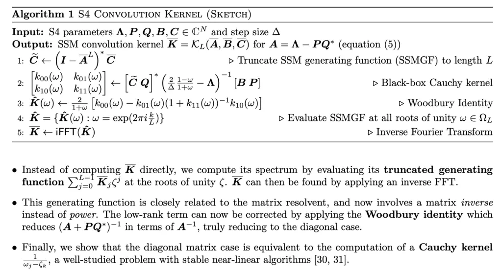

Understanding the specifics of each of these steps is currently above my pay grade, but I will update this page again in the event that I receive enlightenment someday.

The authors then proved that all HiPPO matrices have a NPLR representation, and concludes with a theorem that states that $\oK$ can be computed using only $\tilde{O}(N + L)$ operations and $O(N + L)$ space.

They then showed that this setup results in state-of-the-art performance on many tasks with long-range dependencies, outperforming Transformers and its variants.

Most Glaring Deficiency

In many ways, the S4 model feels reminiscent of a RNN, except it uses a HiPPO matrix for updating its hidden state, which gives rise to opportunities for speedups which is the main focus of this paper.

In this manner, would a traditional RNN approach have performed just as well if the matrix for updating the hidden state was also the HiPPO matrix? This was a question that could have been answered.

It was unclear to me intuitively how the conceptually simple S4 model is somehow capable of capturing long-range dependencies, which plagues regular RNNs. Admittedly this may have been addressed more in-depth in the previous HiPPO paper, but it would make the paper even better if they included some hypotheses on why it works well.

Conclusions for Future Work

This paper showed that state space sequence models can be a viable technique for capturing long-range dependencies in sequential data, by employing a variety of tricks. This technique could inspire future applications that require such capabilities.